
Deep Learning: Image Analysis
FF03 · ©2015 Cloudera, Inc. All rights reserved
This is an applied research report by Cloudera Fast Forward. Originally published in 2015, it features a lot of continually relevant information on how neural networks can be used to interpret images. If you would like more current information on the state of the industry, be sure to check out our updated report on image analysis.
Read the full report below or download the PDF.
Introduction
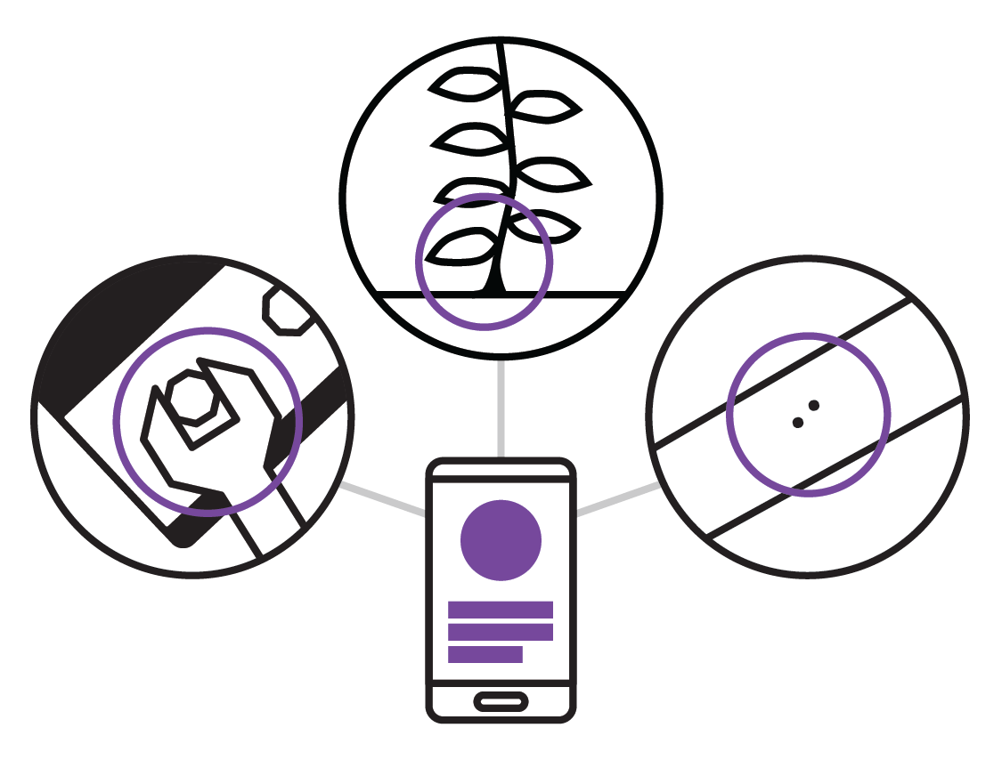
Imagine fixing your car by taking a picture of your engine and having an AI mechanic guide you through the repairs. Or a machine that looks at a rash or bug bite and tells you whether it needs professional attention. Or maybe a program that looks at your garden and warns you which plants are at risk of dying. These ideas may sound like science fiction, but they are now becoming feasible. Recently, we’ve seen massive progress in the development of systems that can automatically identify the objects in images using a technique known as Deep Learning. This is a breakthrough capability.

These systems are emerging now, due to multiple factors. First, there’s been strong progress in our theoretical understanding of artificial neural networks. Neural networks are computational systems made up of individual, interconnected processing nodes that adapt to new input. While they’ve been around since the 1950s, this recent progress has opened up entirely new applications.
Second, graphical processing unit (GPU) computation has become affordable. GPUs were primarily developed for video gaming and similar applications, but are also optimized for exactly the kinds of operations that neural networks require.
Finally, large image and video datasets are now available. This, more than anything, has motivated and enabled significant progress in both research and industry applications. The result is that we are now able to build affordable systems that can analyze rich media (images, audio, and video) and automatically classify them with high accuracy rates.
This has strong implications for anyone building data processing and analytics systems. Current approaches are, out of necessity, largely limited to analysis of text data. This limitation (frequently glossed over by many analytics products) comes from the fact that images can be permuted in many more ways than sentences. Consider that the English language only contains roughly 1,022,000 words, yet each pixel from an image can take on any of 16,777,216 unique color values. Moreover, a single 1024 x 768-pixel image contains as many pixels as Shakespeare had words in all of his plays!
Neural networks, however, are fantastic at dealing with large amounts of complex data because of their ability to internally simplify and generalize their inputs. Already, with high accuracy, we are able train machines to identify common objects in images. It’s exciting to think that we are now able to apply the same kinds of analyses that we’ve been doing on text data to data of all types.
The structure of neural networks was initially inspired by the behavior of neurons in our brains. While the brain analogy is a romantic one, the relationship between these systems and the human brain stops there. These machines do a very good job of solving very specific problems but are not yet able to approach generalized intelligence. We don’t need to worry about the Terminator just yet.
In this report we explore Deep Learning, the latest development in multilayered neural networks. These methods automatically learn abstract representations of their training data to perform some sort of classification or regression task, where you are training a system to look at examples of data with labels and apply those labels to new data. While Deep Learning has implications for many applications, we focus specifically on image analysis because this is one domain where similar results cannot currently be achieved using more traditional machine learning techniques. Deep Learning represents a substantial advancement in image object recognition.

Neural network-based image recognition systems have actually been used in the wild for quite some time. One of the first examples of neural networks applied in a product is the system that recognizes the handwriting on checks deposited into ATMs, automatically figuring out how much money to add into any account.
Image analysis is just the beginning for Deep Learning. In the next few years, we expect to see not only apps that can look at a photo of leaky plumbing or a damaged car and guide you through the repairs, but also apps that offer features such as realtime language translation in videoconferencing and even machines that can diagnose diseases accurately.
Neural Networks
Neural networks have been around for many years, though their popularity has surged recently due to the increasing availability of data and cheap computing power. The perceptron, which currently underpins all neural network architectures, was developed in the 1950s. Convolutional neural networks, the architecture that makes neural image processing useful, were introduced in 1980. However, recently new techniques have been conceived that allow the training of these networks to be possible in a reasonable amount of time and with a reasonable amount of data. These auxiliary algorithmic improvements, in addition to computational improvements with GPUs, are why these methods are only now gaining popularity. Moreover, these methods have proven themselves to excel at extracting meaning from complex datasets in order to properly classify data we didn’t think could be algorithmically classified before.
In this section we’ll look at the basic concepts needed to understand how neural networks function and the recent advances that have greatly expanded their possible applications.
The Perceptron
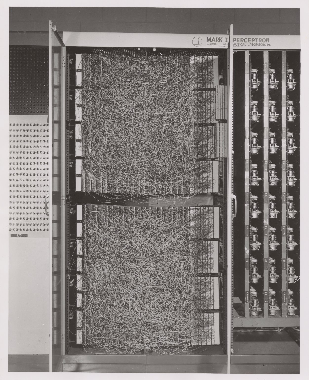
The basic elements of a modern neural network – neurons, weighted connections, and biases – were all present in the first neural network, the “perceptron,” invented by Frank Rosenblatt at Cornell Aeronautical Labs in 1958. The design was grounded in the theory laid out in Donald Hebb’s The Organization of Behavior, which gave a method for quantifying the connectivity of groups of neurons through weights. The initial technology was an array of photodiodes making up an artificial retina that sent its “visual” signal to a single layer of interconnected computing units with modifiable weights. These weights were summed to determine which neurons fired, thus establishing an output signal.
Rosenblatt told the New York Times that this system would be the beginning of computers that could walk, talk, see, write, reproduce themselves, and be conscious of existence. This field has never lacked imagination! Soon researchers realized that these statements were exaggerated given the state of the current technology – it became clear that perceptrons alone were not powerful enough for this sort of computing. However, this did mark a paradigm shift in AI research where models would be trained (non-symbolic AI) instead of working based on a set of preprogrammed heuristics (the Von Neumann architecture).
As the simplest versions of neural networks, understanding how perceptrons operate will provide us insight into the more complex systems popular today. The features of modern networks can be viewed as solutions to the original limitations of perceptrons.
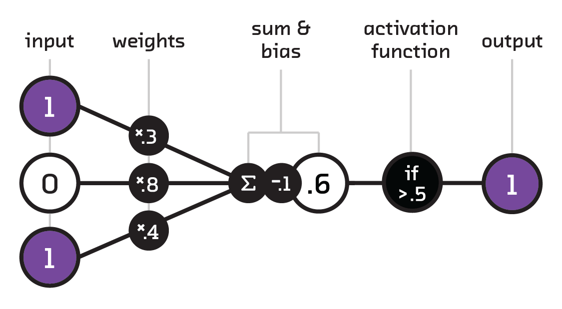
To understand neural networks, we must first unpack the basic terminology: individual computational units (neurons) are connected (i.e., pass information), such that each connection has a weight and each neuron a bias. A number that is passed to a neuron via a connection is multiplied by the weight of that particular connection, summed together with the other inbound connections, and adjusted by the neuron’s bias. This result is passed to an activation function that determines whether the neuron “fires” or not. An active, or fired, neuron passes the result on. If the result does not meet the activation threshold, then it is not passed on.
Perceptrons are simple binary classifiers that use the above computational
components, take in a vector input (see <
The term neuron stems from the biological motivation behind neural nets. A primary property of a brain is its ability to wire (and rewire) neurons together so that, given some input signal (e.g., sound in your ear), groups of neurons will fire together and activate different brain regions, leading to a nervous system or other response. Neurons inside the brain receive input voltages from many connections, but only fire if the current is strong enough to pass across the synapse and carry the electrical signal to them. Similarly, the weights in neural networks allow us to bias certain input connections more than others to extract the relevant features.
Input Vectors
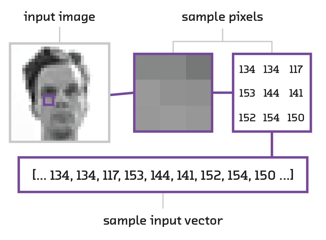
Like most machine learning models, neural networks require an input vector to process. An input vector is a way of quantifying an input as a series of numbers. Neural networks operate by passing this input through layers of neurons that transform the input vector into your desired output.
If we wanted to quantify the properties of a flower as an input vector, we could form a list of numbers describing the flower’s height, the length of the petals, three values for the color (one for each of the red/green/blue values), etc. footnote:[This exact example is part of a classic “hello world” dataset for machine learning called the Iris Dataset.] To quantify words the bag of words approach is generally used, where we create a “master” list in which every possible word has a position (e.g., “hello” could be the 5th word, “goodbye” could be the 29,536th word). Any given passage of text can be quantified using this approach by simply having a list of 0s and 1s, where a 1 represents that that word is present in the passage. An image, on the other hand, is already a quantification of a visual scene – computer image formats are simply 2D lists of pixels, which are just numbers representing the RGB values. However, when creating a vector out of them, we must discard the 2D nature of the data and turn it into a flat list, thus losing any spatial relationships between the pixels.
What makes a perceptron interesting is how it handles weights. To evaluate a perceptron, we multiply each element of the input with a series of weights and then sum them; if the value is above a certain activation threshold, the output of the perceptron is “on.” If the value is below the threshold, the output is “off”:

In this formulation, w encodes the weights being used in the calculation and
is a vector with the same size as the input, x. There is also a bias (also
called a threshold), which is simply a constant number. The result of the
function f(x) defines the classification. That is to say, if we train our
system such that 0 means dog and 1 means cat, then f(a)=0 means that the
data in the vector a represents a dog and f(b)=1 means that b represents a
cat.
While training perceptrons is much simpler than the training regimes we will soon get into, they still do need their weights tuned in order to be useful. For this, we must define a cost function, which essentially defines how far we are from our desired output. We will go into this in more detail soon; for now, it’s useful to know that we are attempting to converge on a result that minimizes our cost function by slowly changing our weights.
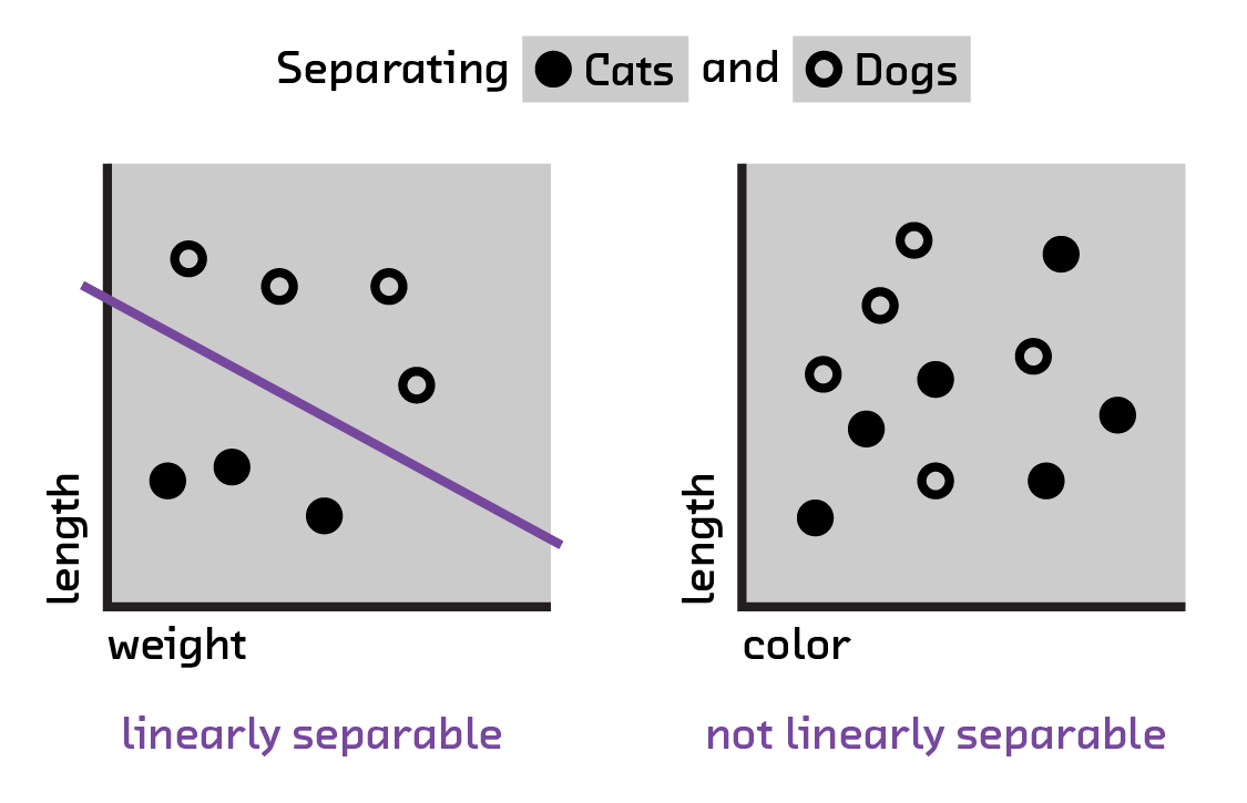
The weights in a perceptron describe a linear function that separates the input parameter space into two sections describing the two possible classifications of the system. As a result, only linearly separable problems can be solved. What we mean by separability is that our parameter space (all features encoded in our input vector) has the capability of having a line drawn through it, which at those values creates a boundary between classes of things. This quickly limits the effectiveness of perceptrons when applied to more complicated classification problems.
=== Feed-Forward Networks: Perceptrons for Real Data ===
As a result of the single layer peceptron being limited to linearly separable problems, researchers soon realized that it could only solve toy problems in its original formulation. What followed were a series of innovations that transformed the perceptron into a model that is still to this day the bread and butter of neural networks: the feed-forward network. This involved the modification of most of the original components, while retaining the underlying theory of Hebbian learning that originally motivated the perceptron’s design.
The feed-forward neural network is the simplest – but most widely used – type of neural network. The model assumes a set of neurons with an arbitrary threshold value and connections to the next set of neurons. The first set of neurons perform a weighted summation of their input; then, that signal is fed forward to the next layer. As connections are unidirectional toward the next layer, the resulting network has no potential cycles, which simplifies the training procedure.
To understand how these networks work, we’ll first need to amend a few of our basic concepts from the perceptron.
==== Nonlinear Activation and Multiple Layers ====
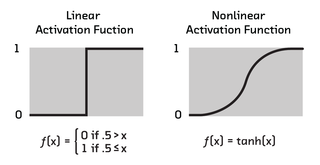
Nonlinear activation functions change several things from the perceptron
model. First, the output of a neuron is no longer only 0 or 1, but any value
from 0 to 1. This is achieved by replacing the piece-wise function that defines
f(x) in the perceptron model with:

where σ is the chosen nonlinear function.[1]
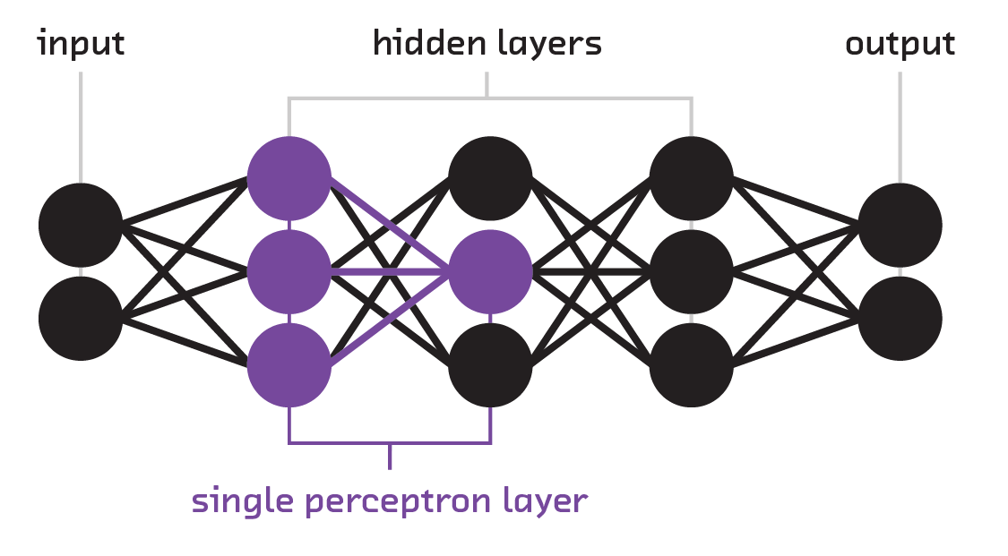
Next, stacking perceptrons allows for hidden layers, at the computational cost of
many more weights. Here, every node in the new layer gets its value by
evaluating f(x) with its own set of weights. As a result, the connection
between a layer of N nodes and M nodes requires M weight vectors of size
N, which can be represented as a matrix of size N x M.
Having multiple layers opened up the possibility of multiclass classification – i.e., classifying more than two items (the limit of the perceptron). The final layer can contain multiple nodes, one for each class we want to classify. The first node, for example, can represent “dog,” the second “cat,” the third “bird,” etc.; the values these nodes take represent the confidence in the classification.
Of course, this introduces the complexity of selecting the correct classification. Should we simply accept the class with the highest confidence, a maximum likelihood approach? Or should we adopt another method (Bayes), where the set of probabilities across all possible classes informs a more sophisticated choice. Maximum likelihood is generally accepted in practice however, in our prototypes we explore alternate methods to make low-confidence classifications useful.
Crucial to these advancements is that they allow classifications of datasets that are not linearly separable. One way to think about this is that the hidden layers perform transformations on the space to form linearly separable results. But the reality is slightly more complicated. In fact, with the addition of nonlinearity, a feed-forward neural network can act as a universal approximator. That is to say, nonlinearity enables a neural network to model any function, with the accuracy proportional to the number of neurons. Adding multiple layers makes it easier to attain high-accuracy models and reduces the total number of required nodes.
Now it begins to come together how adding more layers actually escalates our power to model, classify, and predict. However, why is it that neural networks are so much better then traditional regression and hierarchical modeling? We’ve mentioned before that we train our models; now, let’s take a look at how this is done.
Backpropagation
While these models seem fantastic, it was generally possible to train comparable models on small datasets using classic regression techniques. The real breakthrough for neural networks was in the learning or training procedure: backpropagation. This piece of the puzzle is the reason why neural networks outmuscled previous methods.
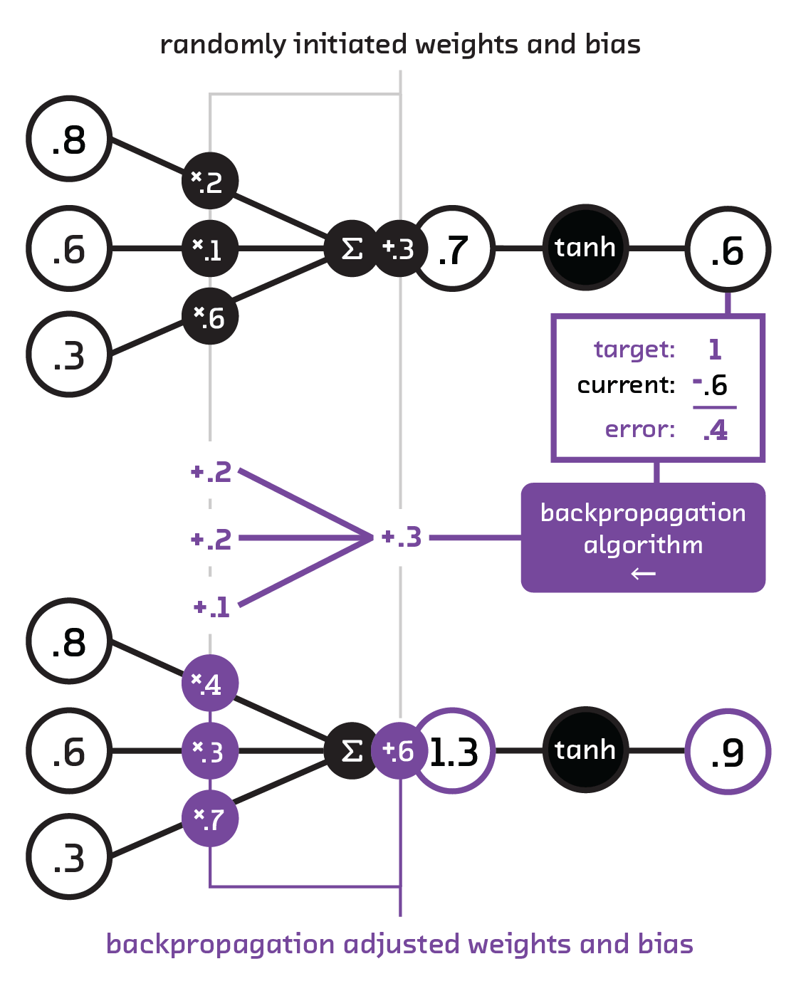
Backpropagation is an optimization technique for models running on labeled data (also known as supervised learning). While this algorithm had been known for quite a long time, it was only first applied to neural networks in 1986. In this technique, data is fed through a randomly initialized network to identify where the network gets things wrong. This error is then “backpropagated” through the network, making subtle changes to gently nudge the weights toward better values. The goal of this training is to craft our weights and biases to transform our input vector, layer by layer, into a separable space (not necessarily linearly separable) where it can be classified. This is done with successive use of the chain rule, which can be thought of as iteratively seeing how much a given weight contributed to a particular result and using the calculated error to correct the problem.
Think of a musician who is playing electric guitar on a new amp for the first time. Her goal will be to make the tonality clear and the distortion appropriate for the song or style, even though the amp’s settings are initially random. To do this, she’ll play a chord with her sound quality goal in mind and then start fiddling with each knob on the amp: gain, mid, bass, etc. By seeing how each knob relates to the sound and repeatedly playing the chord, adjusting, and deciding how much closer she has gotten to her goal, she will do a kind of training. Listening to the chord is like evaluating the objective function, and tuning the knobs is like minimizing the cost function.
While the exact description of the algorithm is outside the scope of this report,[2] there are several
considerations to keep in mind. First, the error that is propagated through the
network is based on the cost function (also known as the loss function).
The cost function defines “how wrong” the neural network was in a given
prediction. For example, if a network was supposed to predict “cat” for a given
image but instead says it thinks 60% it was a cat and 40% that it was a dog, the
loss function would determine how much to penalize the network for the imperfect
output. This is then used to teach the network to perform better in the future.
There are many possible choices for a loss function, and each one penalizes the
network differently based on how incorrect it was versus the correct
output.footnote:[Common loss functions are categorical cross entropy, mean
squared error, mean absolute error, and hinged.] As we’ll see
in <
Second, backpropagation is an iterative algorithm and has a parameter, the
learning rate, that determines how slowly it should change the weights. It is
always advised to start with a small learning rate (generally .001 is used:
if a change of 5.0 would precisely fix the error in the network, a
change of .005 is applied). A small learning rate is crucial to avoid
overfitting the model to the training data because it limits the memorization of
particular inputs. Without this, our networks would learn only features specific
to the training set and would not learn generalization. By limiting the amount the
network can learn from any particular piece of data, we increase the ability of
the network to generalize. This is such an important piece of neural networks
that we even go as far as modifying the cost function and truncating the network
to help with this generalization.
Furthermore, there is no clear time when iterations are done, which can cause
many problems. To address this, we diagnose the network using cross-validation.
Specifically, the dataset should be split into two parts, the training set and
the validation set (generally the training set is 80% and the validation set is 20%
of the data). We use the validation set to calculate an error (also called the
loss), which is compared to the error on the training set. Comparing these two
values gives a good idea of how well the model will work on data in the wild,
since it never learned directly from this validation data. Furthermore, we can
use the amount of error in the training versus the validation sets to diagnose
whether training is complete, whether we need more data, or whether the model is
too complex or too simple (see <
That backpropagation is an iterative algorithm that starts with essentially random weights can also lead to suboptimal network results. We may have terrible luck and initialize our network close to a local minimum (i.e., backpropagation may yield a solution that is better than our initial guess of weights, but nowhere close to a globally “best” solution). To correct this, most researchers train many networks with the same hyperparameters but with different randomly initialized weights, selecting the model with the best result.
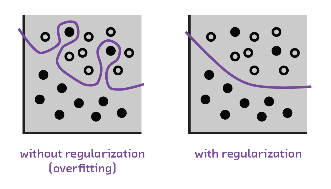
Regularization
Even with our current tools for building neural networks, we still face the basic threat that all machine learning entails: overfitting. That is, even with a complicated architecture, we risk making a neural network that only understands our current dataset. To make sure we don’t teach our pony one trick, we need to create a robust regularization scheme.
Regularization is a set of methods to ensure the model better generalizes from the dataset used to train it. This may not seem as glamorous as finding new neural architectures, but it is just as important since it allows us to train simpler models to learn more complicated classifications without overfitting. Regularization can be applied to a wide range of models, allowing them to perform better and be more robust.[3]
The first form of regularization that was used is L1 and L2 regularization,
collectively known as weight decay (see <[0.4, 0.6, 0.2], we could easily affect
the output vector from that layer using backpropagation; however, the
weights [0.4, 256.0, 0.2] would be almost unaffected by a similarly
backpropagated error. Small weights create a simpler, more powerful model.
A more recent, and very popular, form of regularization called dropout is widely
used. In this method, a random subset of neurons “drop out” of a forward and
backward pass during training. That is to say, with a dropout parameter of
0.2, during training only 80% of neurons are ever used for forward and
backward propagations (and the weight values are scaled accordingly to account
for the reduced number of neurons). As every neuron learns aspects of the
features necessary to do the classification, this means the decision-making
process is spread more evenly across nodes. Think of this as noise being added
to the input, making overfitting rarer since the network never sees the same
exact input twice.
Putting It All Together
In the feed-forward model, we transform the input vector by sending it through neurons that use weights and biases to compute intermediate values. Then we pass these values through a nonlinear activation function to see if the information moves forward. We use multiple layers to allow for more general feature extraction, since each layer gives our model complexity. Finally, we use the result from our output layer to calculate how wrong we were with a cost function. Backpropagation tells us how to adjust each neuron to improve our result, and we use regularization and dropout to generalize our results and prevent overfitting.
This may seem complex, but this background is sufficient to understand, evaluate, and engineer Deep Learning systems.
The feed-forward net is to neural networks what the margarita is to pizza: the foundation for further exploration. Most systems you’ll have encountered in the wild prior to recent innovations were feed-forward neural networks: systems for things like character recognition, stock market prediction, and fingerprint recognition. Having covered the basics, we can now start to take you from simple systems to complex, emergent ones.
Convolutional Neural Networks: Feed-Forward Nets for Images
If Deep Learning ended with feed-forward neural networks, we would have trouble classifying images robustly. So far, our inputs have all been vectors; but images are spatial, intrinsically 2D structures (3D if we include color). What is needed is a neural network that can maintain this spatial structure and still be trained with backpropagation. Luckily, this is exactly how convolutional neural networks work [4].
These networks are quite new. They were first explored in 1980, and
gained wide spread adoption in 1998 in the form of the LeNet (pioneered by Yann LeCun) with their
ability to do hand-written digit recognition. However, in 2003 they were
generalized and simplified
into a form which allowed them to solve much more complex problems.
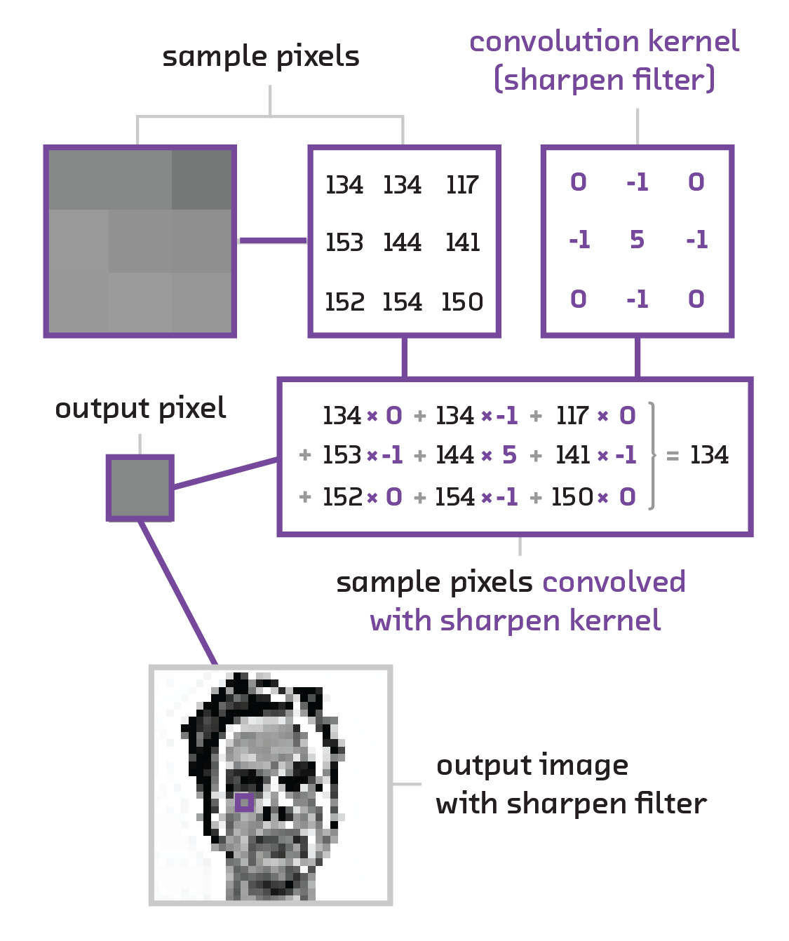
As the name states, instead of operating on the matrix multiplication between the input and a set of weights, a convolutional neural network works on a convolution [5] between the input and a kernel (see below). The kernel is simply a small matrix (generally between 3 x 3 and 8 x 8) that extracts certain spatial features from the image. This sort of technique is used all the time in classical computer image processing. For example, the Sobel operator that is often used for edge detection in images works by convolving a specific set of 3 x 3 matrices with the image. With a convolutional net, we aim to learn the values for these kernels instead of for the full sets of weights.
The full structure of a convolutional neural network is a stacking of several convolutional layers and then several layers of a classic feed-forward neural network. The convolutional layers can be thought of as prepping the data so that the feed-forward layers can take advantage of the spatial structure of the input image. This structure highlights the flexibility of neural networks in general – we can choose to have the convolutional layers feed into a feed-forward neural network or any other type of neural network, depending on what the problem demands. (In 8 The Future we talk about alternate setups used to solve different types of problems, such as captioning images or training a computer to play video games.)
When defining a layer of a convolutional neural network, we specify the number of kernels, how big each kernel is, and the “stride” (step size, or number of spaces moved between each kernel evaluation). This layer will output a new “image” that has a different dimensionality from the input, with spatial features extracted. For example, if our input image was 227 x 227 x 3 (i.e., 227 x 227 pixels over 3 colors) and we used 96 kernels of size 11 x 11 with a stride of 4, the output of this layer would have the dimensions 55 x 55 x 96. These, in fact, are the exact layer parameters for the ImageNet model. In this formulation, each of the 55 x 55 layers is considered a depth slice.
It is important to note that while there are incredibly high numbers of inputs and outputs, there are only 96 x 11 x 11 x 3 weights across the entire layer. With the addition of the 96 biases, this is a total of 34,944 parameters – substantially fewer than the 44,892,219,387 parameters we would have had in a normal feed-forward neural network! This is why convolutional neural networks ushered in neural image processing. It is amazing how much processing can be done with a convolutional neural network given the relatively small number of parameters. The convolutional example above uses the same number of parameters as two feed-forward layers of 186 neurons each, which is quite small for any problem of real interest!
A method known as max pooling, which combines
the values of pixels close to each other, further reduces the number of
parameters in convolutional networks. This can happen on the input or for any
depth slice. Max pooling defines a region, typically 2 x 2- or 3 x 3-pixel
blocks, and only takes the maximum value in any block of that size. This is
similar to downsampling or resizing an image: it both reduces the dimensionality
of the data and adds a form of translational invariance that safeguards the
neural network when the scene is shifted in one direction or another (i.e., if
most pictures of cats have the cat in the center of the image, but we still want
it to perform well if the cat is on the side of the image). We can see the
result of these dimensional reductions in <
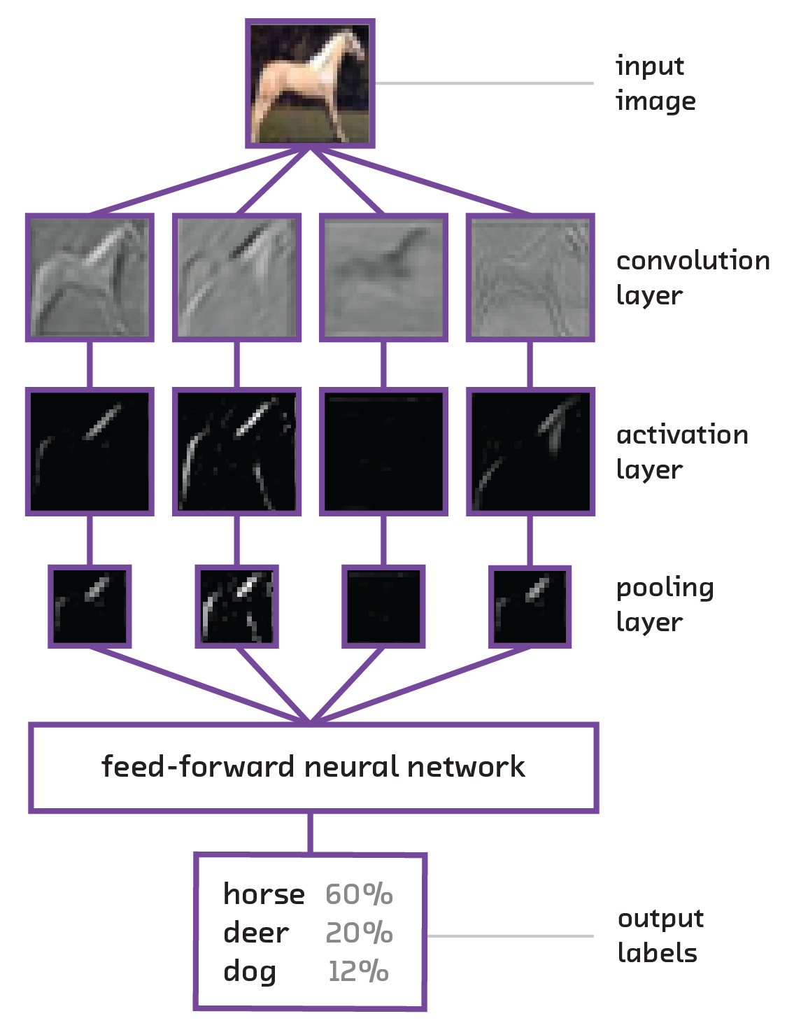
In practice, convolutional networks are used as a feature extractor for classic feed-forward networks. A convolutional neural network takes an image as input and processes it through many layers of convolutions. Once the image has been treated through enough layers, the output of the final convolutional layer is reshaped into a vector and fed into what is called a “fully connected” layer. This may seem like exactly what we were avoiding – once we reshape the data into a vector, we lose the spatial relationships we were trying so hard to maintain. The intuition, however, is that after the image has been passed through multiple convolution steps, the neurons will have been encoded with all the relevant spatial features. For example, if the image had a diagonal edge, there would be some neurons will have encoded that pattern, and therefore rendering the actual spatial data at that point is redundant.
Once in the fully connected layer, we can simply classify as before. In fact, the fully connected region of the network is where we actually start making the associations between the spatial features seen in the image and the actual classifications that we require the network to make. One might think of the convolutional steps as simply learning to look at the picture the right way (i.e., looking for specific color contrasts, edges, shapes, etc.), while the fully connected layers correlate the appearance of particular features with classification classes. In fact, the spatial features seen by the convolutional layers are often robust enough that they can be kept static when training a network on multiple tasks, while only the weights for the fully connected layers are changed from problem to problem in a method called fine-tuning.
Fine-tuning has raised the potential of neural networks as common components within a service. It allows us to use them in transfer tasks: when we take part of a pretrained model and port it over to a different task by fine-tuning the new layers. For convolutional networks, this means we can continue to improve models that encode spatial features while utilizing them in diverse classification problems. Task transfer allows us to iterate on specific pieces of our architecture while modularly building systems for new problems. In many cases, this saves time and computational cost because parts of a robust neural network can be connected into new layers trained around a particular problem.
What Is Deep?
Having taken the long walk with us through the building blocks of this technology, you may still be wondering, “What exactly is this Deep Learning thing?” Since you’re likely to hear this term trumpeted by many new companies and the media in the near future, we want to make sure it’s given some context – or should we say, depth.
As previously shown, layers in a neural network can be stacked as desired, at the cost of computation and the requirement for more data. However, with each new layer, the neural network is able to create more robust internal representations of the data. This can allow a deep neural network to tease out very subtle features from the data to accurately classify inputs that would cause other models to fail.
It is important to realize, however, that when we speak of “deep” learning, we are not simply referring to the number of layers. While there is no concrete definition of what “deep” means in this context, it is generally accepted that the number of causal connections each neuron has is a more accurate representation of the depth. That is to say, if a particular neuron’s output can affect a large number of other neurons through many possible paths, that network is considered deep. [6] This focus on the number of possible causal connections allows us to think of powerful but small architectures as deep. For example, simple two-layer recurrent neural networks may not have many layers, but the robustness of the neural connections creates many causal links, resulting in a network that can be seen as very deep.
What Neural Networks Are and Are Not
The very term “neural network” invokes cybernetic imagery. We easily fall into the old sci-fi fantasy of thinking, conscious machinery. While seductive, this account of what a neural network is doing is practically entirely false. Neural networks are structurally and functionally dissimilar from real brains, even if the brain’s neural connectivity inspired the computational infrastructure.
In this section, we’ll develop intuition around what tasks neural networks succeed at and debunk the mythology around these “artificial brains.” With this knowledge, we can evaluate why they aren’t quite brains, but still do an impressive job of modeling highly complex functions that can classify large and diverse data – and, importantly, learn how to identify when claims around neural networks are being overstated.
Interpreting a Neural Network
In Section 2, we covered the basic architecture and computational techniques used to design and train neural networks. How computer scientists often interpret these systems is that we are creating one glorified feature extractor. That is, we comprehend our data as having discrete features that, once teased out, tell us how that data should be treated given some classification or prediction goal. This is the assumption of separability that essentially means we believe our data’s features can be identified, separated, and bounded so as to make robust class distinctions. Neural networks are tools for extracting out these features and, in turn, making classification decisions.
You may remember that with convolutional neural networks (which are used for object recognition), we use kernels to encode features from smaller sections of our images (e.g., detecting an edge). With these features encoded, we can then use further layers to separate our feature space. And this is the essence of even the most complicated, multilayered neural networks: layer by layer we are transforming our data, first to encode the data’s features and then to filter them based on how our model has “learned” to categorize those features. Because these transformations are nonlinear and we do not actually know what features each layer is encoding, any further interpretation requires a very fine, technical inspection of the model in action.
Due to this complexity, many researchers have worked on visual techniques that give them insight into what is happening at each layer. [7] There are many people who specialize in gaining practical results (e.g., tuning hyperparameters, adding/subtracting layers), but this high-level description is about as close as we get to interpreting what these systems are actually doing.
Some of you may have seen the images generated by Google’s Deep Dream software, which incepts images with psychedelic-looking dogs, buildings, etc. [8] This technique was designed to gain insight into what the neural network is encoding at a particular layer. The tactic is to take an already trained network but only evaluate it up to the layer we want to inspect. Then, taking a separate image that we want to “incept” into our neural network, we run our inception image up to the layer we want to inspect and get its values. Then we run our backpropagation algorithm, except instead of minimizing our usual cost function, we minimize against the values found for the incepted image. Finally, we backpropagate all the way into the image, treating it as a modifiable layer rather than fixed input data, adjusting its pixel values to get a visual representation of what it’s trying to encode.
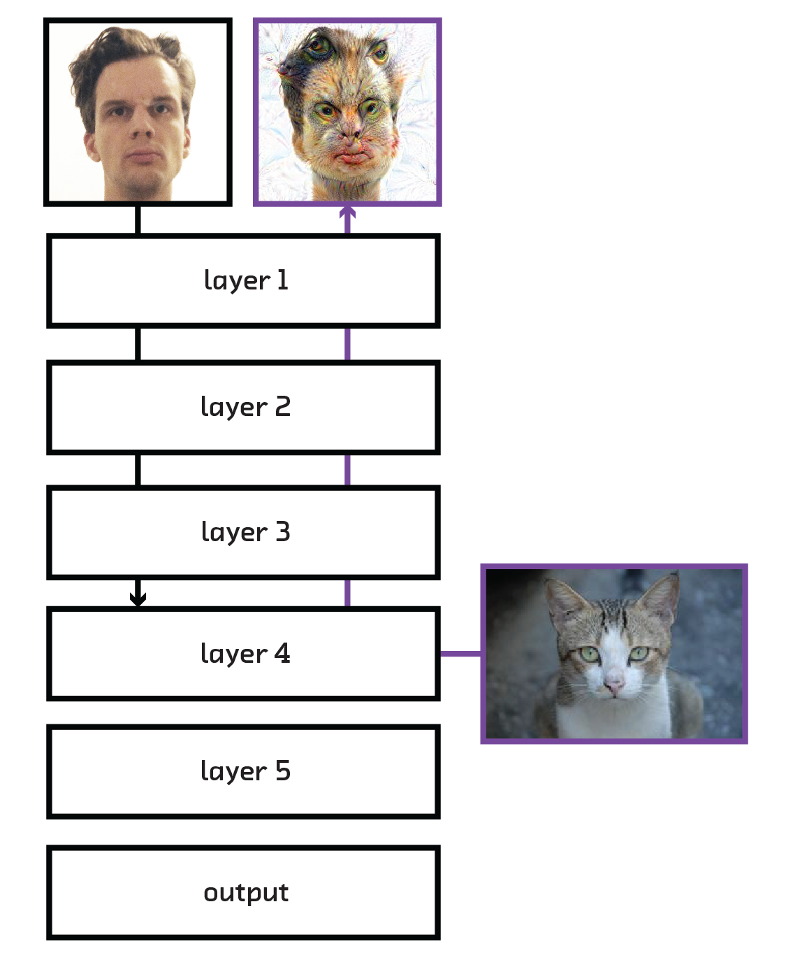
While this method may seem like a toy and nothing else, it provided us with the
first insight into the complexity of the features that a convolutional neural
network was using to do its classification. Before, the only way to see what
features were being extracted was to look at the activation maps (see
<
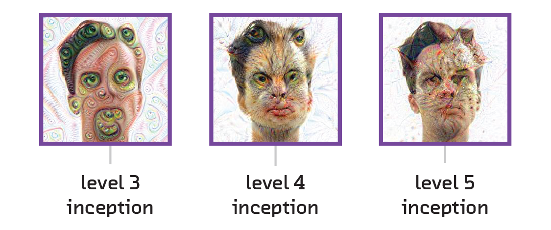
Google’s method is a taste of how one may be creative in figuring out what a neural network is encoding. It is only good for visual images, and tells us a limited amount, but it allows us a visual – and sometimes creepy – insight into what the weights and biases of a particular layer mean.
Limitations
For someone who makes plans and decisions based on emerging technologies, it is crucial to have a discerning eye for what is achievable and what is far-fetched. Having now seen the basic concepts behind neural networks and a functional interpretation, you may already have some inkling as to why these systems are not “strong AI.” [9] While neural networks are powerful, the brain-like vocabulary is misleading. Obviously, they are materially different, but these systems are not “brains” from a functional standpoint either.
To begin with, brains have plastic connections – neuron A may not always be connected to neuron B at all times – whereas in neural networks these connections are rigidly defined. Further, in brains, everything is a function: even activation functions are functions since neuronal activations are primed by many conditions determined by the local chemical state. Neural inhibitors and transmitters modify individual synapses, changing both the firing potential and the signals transmitted. Rather than accepting input vectors of a specific shape, brains adapt to multimodal inputs that are combined internally.
All of these functional differences must be taken seriously before we go too far in comparing neural networks to human intelligence. These descriptions tell us what’s different, yet only go so far in characterizing what they amount to in the way of limitations. Many of the tasks that we are eager to see AI accomplish involve cognitive criteria for success. Understanding this distinction between cognitive and computational involves clarifying the difference between learning and thinking, as well as processing and integrating information.
As was elaborated in Section 2, neural networks have a capacity for learning via parameter adjustment. Recall that this learning is the result of minimizing a single objective function defining our task. The existence of the objective function makes learning in neural networks quite different from in brains. Why we will distinguish the role of thinking to understand this contrast is because the process of thinking involves switching and integrating contexts – something neural networks are not yet able to do. Here, learning is the feedback system that improves practical results on a task, whereas thinking is the process that reflects on the task, our goal orientation toward it, the varying approaches we may take, etc. In neural network terms, this would imply objective functions constantly morphing (task redefinition) and the shape of input vectors changing (context adjustment) as needed. Consider being taught a word, but then asking your teacher for a visual demonstration to go along with the syntactic definition – both the visual and auditory contexts aid in your learning. Neural networks do not have this flexibility.
An implication of how neural networks are currently designed is that they are processing systems rather than integrating systems. That is, they do not know or care about outside information that may be pertinent to their task, or about whether their goal is appropriate. They merely act on particular input shapes, achieving particular output shapes using rigidly defined computations. An integrating system requires a higher-order functioning that cannot be reduced to any particular processing task, which itself can include/exclude specific information and adjust the task. It is integration that is needed for cognitive tasks and that must be worked on before AI encroaches on the kind of intelligence we dream about in our sci-fi fantasies – strong AI.
With that said, we still find neural networks extremely useful because they allow us to take a diversity of inputs and model arbitrarily complex functions. Given that developing functions for mapping intricate inputs into simple outputs is an extremely difficult task, neural networks offer technologists an incredible service by being able to approximate any continuous function capable of being written down. We call this the universality of neural networks, and it will be touched on in the next section.
Common Misconceptions
Despite the limitations characterized above, neural networks continue to be in the press with many fantastical articles written about them. It seems that every week a new neural network is devised that reportedly gets closer and closer to being able to read your thoughts or interact with you in a deeply personal way. However, as you now know, these claims are far from the truth. While neural networks are indeed advancing, we are at a point where either vast improvements must be made to the algorithms or we must devise exponentially bigger computers. [10]
This is because current neural networks are quite limited in the generality they can obtain. We are only now reaching levels where image classification can be done at an accuracy better than that achievable by humans; however, that is only for a very focused set of classification labels on a very curated dataset (known as the ImageNet dataset, which is used annually in image recognition competitions).
It has been shown, however, that neural networks do very well on transfer tasks, where the model has been trained on one problem and is then applied to a different problem with minimal retraining. However, just as before, these tasks must have quantifiable objectives, making them very limited in scope – a limitation currently affected by the sizes of both the models and the datasets we have available to train on.
Furthermore, an aspect of neural networks that is often left undiscussed in public is how the exact formulation of the data determines our effectiveness. We may feel tempted to believe that if we had a large enough neural network and all of Facebook’s data, we could predict users’ preferences given certain online actions. This misconception stems from the nature of training on cost functions, since neural networks currently only show their real utility for supervised learning problems where the correct results are known for the given training set. That is, to train the neural network we must have a labeled dataset that teaches the model correct relationships between input and desired output.
This problem with datasets can also lead to many subtleties where a dataset does indeed exist, but is not robust enough to fully describe the problem. For example, if we had images of news anchors as they were talking about different stories, and each image was labeled with the topic of the story the person was discussing, would we be able to later determine the topic of a story given an image of the news anchor? This might be possible in certain cases – for example, if the topic was weather we could probably use the existence of a weather map in the background as a giveaway. However, for many other topics there are no cues that could be used to determine what is being talked about, since we are simply using the wrong data – we are using images of the anchor when what we really want is audio or a transcription of what is being discussed! This type of problem is quite prevalent, where it seems our dataset has the right association, but it is missing the correct context in order to find a reasonable solution to the problem.
In the end, neural networks are not magical devices that can solve any problem they are given. Instead, they are a way of training incredibly large models to solve very high dimensional problems. So as you consider whether or not they are right given your problem, or whether to believe someone else’s claim to be solving a problem using a neural network, here’s a list of questions to ask yourself:
- Can you quantitatively describe the features of your problem space?
- Does the problem always require the same information to solve?
- If you were to give this task to a group of humans, would you expect consensus?
- Is the problem’s solution context dependent? If so, does the data cover that context?
- Can you verify the correctness of a given output?
- Does the neural network claim to know you better than you know yourself?
Are Neural Networks Right for You?
There are many things to consider when deciding whether to use neural networks in your system. While very powerful, they can also be very resource intensive to implement and to deploy. As a result, it is important to make sure that other options have already been exhausted. Trying simpler methods on a given problem will at the very least serve as a good benchmark when validating the effectiveness of the neural model. However, for images, non-neural methods are quite limited unless auxiliary data is available (for example, quality-controlled user-generated tags with standard clustering and classification algorithms could be a good first-pass solution).
Picking a Good Model
If a neural model seems like the only solution, one of the most important considerations when starting is whether a model (particularly a trained model) that solves the problem already exists. These pretrained models have the advantage of being ready to use immediately for testing and already having a predefined accuracy on a given dataset, which may be good enough to solve the problem at hand. Getting to those accuracies often involves tuning many parameters of the model, called hyperparameters; this can be quite tedious and time-consuming, and requires expert-level understanding of how the model works in order to do correctly. Even with all other hurdles taken care of, simply figuring out a good set of hyperparameter values for the model can determine whether the resulting model will be usable or not.
There are many pretrained models out there to use. Caffe, for example, provides
a model zoo where people can share models in a standardized way so they can be
easily used. One that is of particular interest is the googlenet model, which
comes with an unrestricted license and does ImageNet classification, out of the
box, with 68.7% accuracy for predicting the correct tag and 89% accuracy for
having the correct tag in the top five results. While some of the models in the
zoo are released under a commercial-friendly license, many are distributed using
a non-commercial license (normally as a result of restrictions on the underlying
dataset). However, these pretrained models can at least serve as a good basis
for testing to see if the particular approach is valid for your problem before
going ahead and training the same model on your own custom data.
Notable Models in the Model Zoo
- Places-CNN: Trained on images of various locations and of various objects
- FCN-Xs: Segments images to find the locations of objects in images
- Salient Object Subitizing: Finds the number of objects in an image
- Binary Hash Codes: Generates semantic image hash codes for fast “similar image” retrieval
- Age/Gender: Predicts the age and gender of a person through an image
- Car Identification: Identifies the model of a car
Fine Tuning / Transfer Learning
Once a pretrained model is found, it can either be used outright or run through a process called fine-tuning [11]. In fine-tuning, a pretrained model is used to initialize the values for a new model that is trained on new data. This process shows how robust neural networks can be – a model trained for one purpose can very easily be converted to solving another problem. For example, a model used to classify images can be fine-tuned in order to rank Flickr images based on their style [12]. A benefit of this is that the pretrained model already has some abilities in recognizing images, or whatever task it was intended for, which means the fine-tuning training is more focused and can be done with much less data. For applications where a pretrained model that solves the given problem cannot be found, and an adequately sized dataset is not available, it may be necessary to find a “good enough” pretrained model and use fine-tuning to repurpose it for the given problem. As mentioned in the description of <<convnet,convolutional neural networks>>, often convolutional layers are reused since their ability to extract objects from a scene are not necessarily greatly affected when changing the downstream classification task at hand. [13]
Datasets and Training
One of the biggest difficulties with training your own neural network is finding a large enough dataset that fits the problem space. While deep neural networks can be trained to perform a wide variety of tasks, as more layers are added (and thus the total number of parameters of the model increases), the amount of data necessary for training also increases. As a result, when deciding whether it is possible to train your own neural network to solve a problem, you must consider two main questions: “Do I have enough data?” and “Is my data clean and robust enough?”
Unfortunately, there are no easy ways to know a priori whether your dataset is large enough for the given problem. Each problem introduces its own subtleties that the neural network must learn to figure out – the subtler the differences between the example data, the more examples are necessary before the model can figure them out.
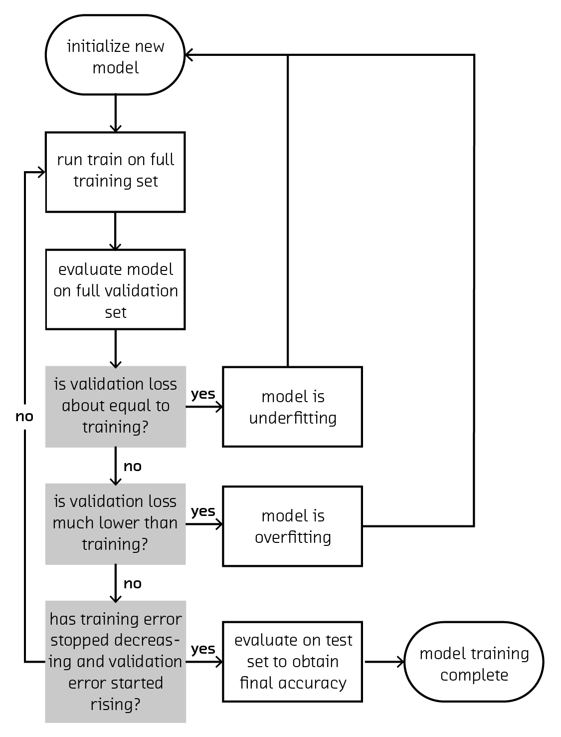
A good rule of thumb is to compare the results of your cost function between the training and validation sets, also known as training loss and validation loss. Commonly we aim at having a training loss that is a bit higher than the validation loss when performing backpropagation. If the training loss is about the same as the validation loss, then your model is underfitting, which means you should increase the complexity of the model, adding layers or connections. If the training loss is much lower than the validation loss, then your model may be overfitting. Solutions to this include decreasing the model’s complexity or increasing the dataset size (synthetically or otherwise).
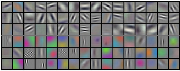
Furthermore, when training a convolutional neural network, it is useful to look at the actual kernels to gauge the performance of the network while it’s being trained. We expect the kernels to be smooth and not look noisy. The smoothness of the resulting kernels is a good measure of how well the network has converged on a set of features. Noisy kernels could result from noisy data, insufficient data, an overly complex model, or insufficient training time.
One common way to synthetically increase the dataset size in an image-based task is through multisampling, where each image is cropped in multiple ways and flipped horizontally and vertically. Sometimes, noise is even introduced into the input every time a piece of data is being shown to the network. This method is recommended in every application, not only because it increases the dataset size, but also because it makes the resulting network more robust for rotated and zoomed-in images. Alternatively, the dropout method discussed in Section 2 (a type of regularization) can be used. It is generally advisable to always use the dropout method with a small dropout factor to prevent overfitting whenever there is limited data available.
However, if tweaking the model complexity, dataset size, or regularization parameters doesn’t fix the validation and training losses, then your dataset may not be robust enough. This can happen if there are many examples of one category but not many of another (say, 1,000 images of cats but only 5 of scissors), or if there is a general asymmetry in the data that allows the neural network to learn auxiliary features. A common example of this in image training is the picture’s exposure and saturation. If all pictures of cats are done using professional photography equipment and pictures of scissors are taken on phones, the network will simply learn to classify high-quality images as cats. This problem shows itself quite often in the use of pretrained networks on social media data – many pretrained networks use stock photography as their training set since it is highly available, however there are vast differences between the quality and subject of stock pictures and pictures found on social media websites. One solution is normalizing images, a procedure where the mean pixel value of the entire dataset is subtracted from each image in order to deal with saturation and color issues. However, in cases where the dataset the model is being applied to differs drastically from the training set, it may be necessary to fine-tune the model, or start from scratch.
Testing What You’ve Made
Finally, it is important to understand the model you have created or intend to use. Even though neural networks are non-interpretable models (meaning we cannot gain too much insight into the internals of how the model is making the decisions it is), we can at least understand the domain that the model is applicable for by looking at the training set and having a robust enough test set.
For example, if we create a network that can estimate the amount of damage done to a region by a natural disaster using satellite imagery, what will the model say for regions that were completely unaffected? Is it biased to specific architectural or geographical features because of a bias in the dataset? Or maybe those biases simply emerged because the model was not robust enough to extract deeper features. Having a holdout sample of the dataset that is only used once the model is fully trained can be invaluable in understanding these sorts of behaviors; however, a careful analysis of the dataset itself is important.
Furthermore, consideration must be given to cases where the neural network fails to give a high-confidence result, or simply gives the wrong result entirely. Currently, accuracies of >85% at image processing tasks are considered cutting edge; however, this means that for any high-volume application many incorrect results are being given. Results from a neural network also come with confidences, so a threshold in quality should be recognized for the given task and downstream applications should have procedures for when no results match the given confidence level. Another route is to use the results of the neural network to inform further algorithms in a way that can potentially increase the confidence, or at least the usability, of the results. In our prototypes, we use a hierarchical clustering on the predicted labels in order to increase the usability of low-confidence results. This draws on the intuition that even if an image cannot be confidently classified as a cat, most of the labels with nonzero confidences will be under the WordNet label “animal,” and this is a sufficiently informative label to use in this case.
Timelines
Below are some suggested timelines for working with neural networks in different situations. It is important to note that these numbers are incredibly approximate and depend very much on the problem that is being solved. We describe a problem as a “solved problem” if there already exists a pretrained model that does the specified task.
| Situation | Research | Data Acquisition | Training | Testing |
|---|---|---|---|---|
| Pre-Trained Model Available | 1 week | days | N/A | 1 week |
| Similar to Pre-Trained Model | 1 week | 1 week | days | 1 week |
| Similar to Problem in a Paper | weeks | 1 week | 1 week | 1 week |
| New application of known model | weeks | 1 week | weeks | 1 week |
| New application and novel model | months | weeks | months | weeks |
Deploying
Deploying a neural network is relatively easy; however, it can be quite
expensive. The trained model is large – easily 500 MB for a single moderately
sized network. This means that git is no longer an adequate tool for
versioning and packaging the datafile, and other means should be used. In the
past, using filename-versioned models on Amazon’s S3 has worked quite well,
particularly when done with the S3 backend for git-annex.
The machine that the model gets deployed on should have a GPU and be properly
configured to run mathematical operations on it. This can be difficult initially
to set up; however, once installed correctly, backups of the machine can easily
be swapped in and out [14].
The main complication comes from installing cuda if you are using an NVIDIA
device, as well as installing cuda-enabled math libraries such as theano,
caffe, cudnn, cufft, etc.
Once the model file is on a machine properly configured to use its GPU, using the neural model is quite the same as using any other model. A common route for facilitating a distributed cluster of these models is to wrap the network itself in a thin lightweight HTTP API and deploy it to a cluster of GPU-enabled machines. Then, any service in your ecosystem that must take advantage of the model’s power can pick a server in this cluster using a round-robin approach – new models can be uploaded and, one by one, computers in the neural network cluster can be updated without disrupting downstream services.
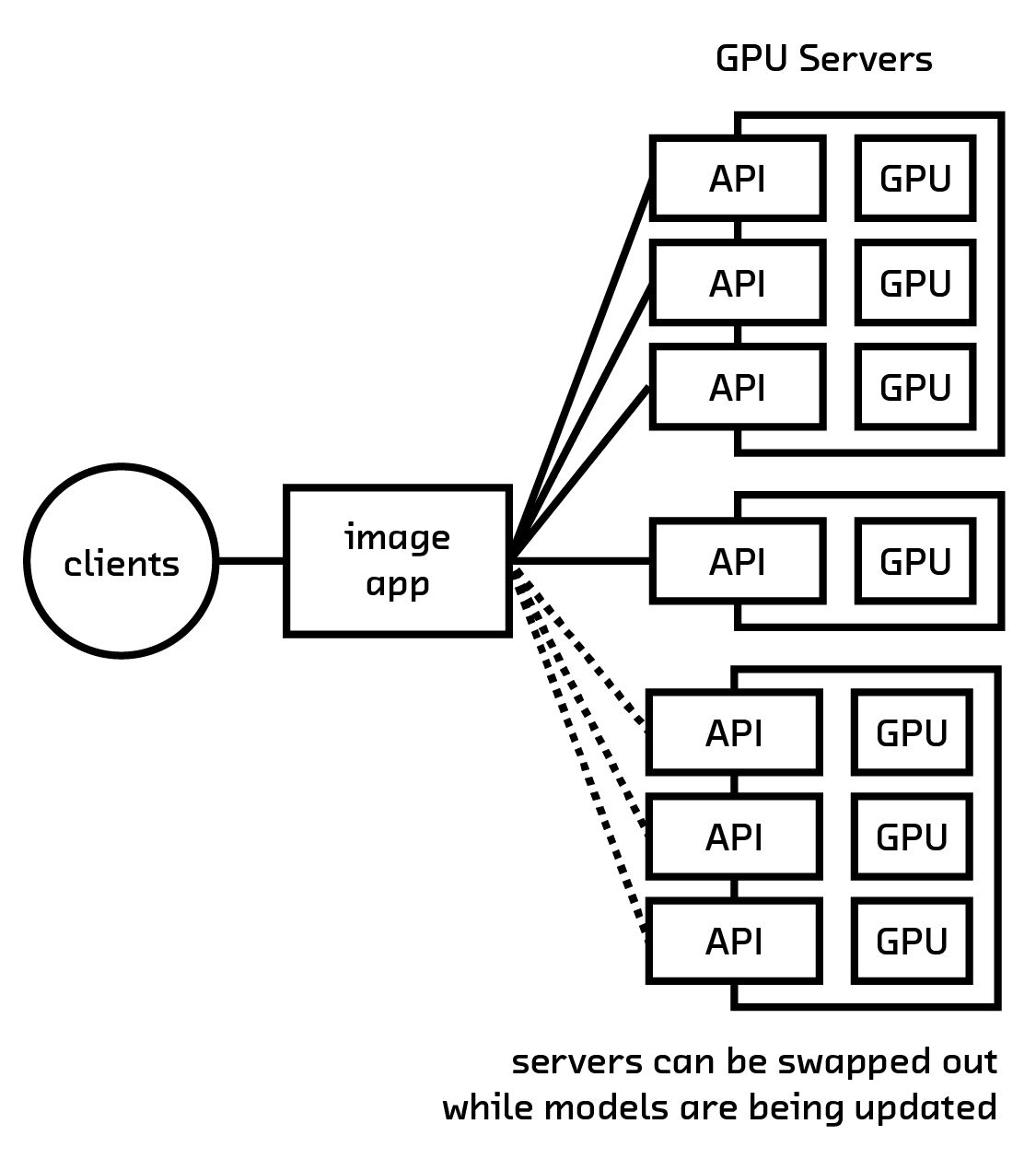
Having a policy for rolling out new models is quite important. Models generally need to be updated as their usage changes and new/different datasets become available that could increase their accuracy. It is very much suggested to instrument any service that uses the results of the neural network in order to obtain feedback data for use in future training (for example, asking the user “Was our result good?” or “What better response could we have provided?”).
Hardware
As described in 2 Neural Networks, while we think of these models as a series
of neurons connected to each other with various activation functions, the
results are actually computed with a series of vector operations. In fact, most
neural networks can be seen as simply taking the linear combination of vectors,
applying some nonlinear function (a popular choice is the tanh function), and
maybe taking a Fourier transform. These computations are perfectly suited for a
GPU, which has been optimized at the hardware level to perform linear algebra at
high speeds.
This is why NVIDIA has been very strongly pushing for using its GPUs for general mathematics as opposed to simply gaming. They have even gone as far as creating very specialized math libraries that optimize these linear algebra operations on their devices and, in recent months, developing specialized neural network hardware for their next-generation, computation-specific GPUs.
These considerations have gone from being useful for the academic working on
these problems to necessary for anyone working with neural networks – our
models are getting more and more complex, and the CPU is no longer adequate for
training or evaluating them. As a result, infrastructure using neural models
must have GPUs in order to function at acceptable speeds. When working on
Pictograph, we found that we could perform a single image classification in
about 6 seconds on the CPU, vs. 300 ms on the GPU (using the g2.2xlarge AWS
instance). Furthermore, the operations scale very well on a GPU (often
incurring almost no overhead if multiple images are classified together).
Deep Learning in Industry Today
Neural networks have been deployed in the wild for years, but new progress in Deep Learning has enabled a new generation of products at startups, established companies, and in the open source community.
In the startup community we’ve seen several companies emerge with the aim of making Deep Learning affordable and approachable for any product manager or engineer, as well as companies that apply Deep Learning to a specific problem domain, such as medicine or security. There’s been similar growth in the open source community, as companies and academics contribute code back to a variety of libraries and software packages.
Current applications of Deep Learning in industry include voice recognition, realtime translation, face recognition, video analysis, demographic identification, and tagging. We expect this flourishing of new development to continue over the next couple of years as new applications are discovered, more data assets appropriate to Deep Learning become available, and GPUs become even more affordable.
Commercial Uses of Deep Learning
The current enthusiasm for Deep Learning was spawned by a 2012 paper from Google [15] describing how researchers trained a neural network classifier on extremely large amounts of data to recognize cats (many examples used for illustration purposes in this paper is a nod to these researchers) Since then, big players like Google, Microsoft, Baidu, Facebook, and Yahoo! have been using Deep Learning for a variety of applications.
All of these companies have a natural advantage in creating Deep Learning systems – massive, high-quality datasets. They also have expertise in managing distributed computing infrastructure, giving them an advantage in applying Deep Learning techniques to real-world problems.
Google has published a follow-up to its 2012 paper [16], and is now using Deep Learning for realtime language translation, among other things. Its recent announcement of a realtime voice translation service on mobile phones is impressive both for the functionality [17] and for the application architecture – it runs on a standard smartphone.
Facebook formed FAIR,[18] the Facebook Artificial Intelligence Research Lab, in 2013, and hired Yann LeCun, one of the pioneers of Deep Learning research and a professor at NYU, as its director. FAIR has developed face recognition technology that has been deployed into an application that allows Facebook users to organize personal photos and share them with friends, [19] and contributed to numerous open source and academic projects. FAIR operates from Facebook’s New York Astor Place office, Menlo Park, CA, and Paris.
Baidu hired Andrew Ng, coauthor of the Google cat paper and Stanford professor, to lead their Deep Learning research lab out of Cupertino, CA. Baidu’s Minwa system is a purpose-built Deep Learning machine for object recognition.
Yahoo! is using image classification to automatically enrich the metadata on Flickr, its social photo site, by adding machine-generated tags to every photo. [20]
The relationships between researchers and companies are complex because these techniques emerged from a small and tight-knit research community that has recently exploded into relevance, with this obscure research area becoming one of the hottest areas for hiring among the Internet giants. Ideas that may have begun at one institution show up in applications developed by another, and people often move between institutions.
Deep Learning as a Service
If you are considering using Deep Learning but don’t plan to develop and train your own models, this section provides a guide to companies that offer services, generally through an API, that you can integrate into your products.
Clarifai
Clarifai [21] is a New York-based startup that uses Deep Learning to recognize objects in still images and video data. Clarifai’s models won the 2013 ImageNet competition.
Clarifai’s API allows users to submit an image or video, then returns a set of probability-weighted tags describing the objects recognized in the image or video and the system’s confidence in each tag. The API can also use an image input to find similar images. It runs quickly; it is capable of identifying objects in video streams faster than the video plays.
Founder Matthew Zeiler says, “Clarifai is building products that empower people to understand the massive amounts of information they are exposed to daily, making it easy to automatically organize, analyze, and share.”
Dextro
New York-based Dextro [22] offers a service that analyzes video content to extract a high-level categorization as well as a fine-grained visual timeline of the key concepts that appear onscreen. Dextro powers discovery, search, curation, and explicit content moderation for companies that work with large volumes of video.
Dextro’s models are built specifically for the sight, sound, and motion of video; its API accepts prerecorded videos or live streams, and outputs JSON objects of identified concepts and scenes with a timeline of their visibility and how prominent they were onscreen. Dextro can output in IAB Tier 2, Dextro’s own taxonomy, or any partner taxonomy.
Dextro offers a great service for any company that has an archive of video content or live streams that they would like to make searchable, discoverable, and useful.
David Luan, cofounder of Dextro, describes it as follows: “Dextro is focused on immediate customer use cases in real-world video, and excels at user-generated content. Our product roadmap is driven by our users; we automatically train large batches of new concepts every week based on what our partners ask for.”
CloudSight
CloudSight ^cloudsightapi.com/] is a Los Angeles-based company focusing on image recognition and visual search. Their primary offering is an API that accepts images and returns items that are identified in those images. They also use this API to power two apps of their own: TapTapSee, which helps visually impaired uses navigate using their mobile phones, and CamFind, which is a mobile visual search tool where users can submit images from their cameras as queries.
[[FIG-cloudsight]] .CloudSight recognizes a puppy image::figures/cloudsight_beagle.png[scaledwidth=“90%”]
MetaMind
MetaMind [23] offers products that use recursive neural networks and natural language processing for sentiment analysis, image object recognition (especially food), and semantic similarity analysis. MetaMind is located in Palo Alto, CA, and employs a number of former Stanford academics, including its founder and CEO, Richard Socher. It raised $8 million of capital in December 2014.
Dato
Dato [24] is a machine learning platform targeted at data scientists and engineers. It includes components that make it simple to integrate Deep Learning as well as other machine learning approaches to classification problems.
Dato doesn’t expose its models, so you are not always certain what code, exactly, is running. However, it offers fantastic speed compared to other benchmarks. It’s a good tool for data scientists and engineers who want a fast, reliable model-in-a-box.
LTU Technologies
LTU Technologies [25] is an image search company founded in 1999 that offers a suite of products that search for similar images and can detect differences in similar images. For example, searching a newspaper page from two different dates may reveal two advertisements that are similar except for the prices of the advertised product. LTU Technologies’ software is also geared toward brand and copyright tracking.
Nervana Systems
Nervana Systems [26] offers a cloud hardware/software solution for Deep Learning. Nervana also maintains an open source Deep Learning framework called Neon [27], which they describe as the fastest available. Notably, Neon includes hyperparameter optimization, which simplifies tuning of the model. Based in San Diego, Nervana was founded in April 2014 and quickly raised a $3.3 million Series A round of capital.
Skymind
Skymind [28] is a startup founded by Adam Gibson, who wrote the open source package DeepLearning4j [29]. Skymind provides support for enterprise companies that use DeepLearning4j in commercial applications. Skymind refers to itself as “The Red Hat of Open-Source AI for Enterprise.”
Unlike other startups listed here, Skymind does not provide service in the form of an API. Rather, it provides an entire general-purpose Deep Learning framework to be run with Hadoop or with Amazon Web Services Spark GPU systems. The framework itself is free; Skymind sells support to help deploy and maintain the framework. Skymind claims that DeepLearning4j is usable for voice-to-text tasks, object and face recognition, fraud detection, and text analysis.
Recently acquired startups
There have recently been many acquisitions of startups using Deep Learning technology. These include Skybox Imaging (acquired by Google), Jetpac (also acquired by Google), Lookflow (acquired by Yahoo!), AlchemyAPI (acquired by IBM), Madbits (acquired by Twitter), and Whetlab (also acquired by Twitter).
The challenges for independent Deep Learning startups include attracting the necessary talent (generally PhDs with expertise in neural networks and computer vision), accessing a suitably large and clean dataset, and finally figuring out a business model that leads to a reasonable monetization of their technology. Given these challenges, it’s not surprising that many small companies choose to continue their missions inside of larger organizations.
Startups Applying Deep Learning to a Specific Domain
Many entrepreneurs are excited about the potential of Deep Learning and are building products that have only recently become possible because of the accessibility of these techniques.
Healthcare
Healthcare applications push the boundaries of machine learning with large datasets and a tempting market with a real impact.
Enlitic [30], a San Francisco-based startup, uses Deep Learning for medical diagnostics, focusing on radiology data. Deep Learning is fitting for this application because a Deep Learning system can analyze more information than a doctor has ready access to, and may notice subtleties that are not clear to humans.
Atomwise [31] is a Canadian startup with offices in San Francisco that focuses on using Deep Learning to identify new drug candidates, and Deep Genomics [32] focuses on computational genomics and biomolecule generation.
For quite a long time, analysis of text records has been used to improve the patient experience and expand the knowledge available to doctors and nurses. However, that information is severely limited in scope and detail, simply as a result of being a burden to maintain for doctors. The ability to automatically encode the information in images such as x-ray and MRI scans into these records would provide a valuable additional source of data, without placing an added burden on the healthcare practitioners.
Security
The security domain offers subtle pattern recognition problems. Is this server failing? Is that one being compromised by unusual external activity? Deep learning is a fantastic mechanism for this sort of problem since it can be trained to understand what “normal operating conditions” are and alert when something deviates from it (regardless of whether the operators knew whether to intentionally put in a rule or heuristic for it). For this reason, neural networks have even been used as a backup system to monitor the safety of nuclear facilities. As a result, there has been progress in both academic research [33] and industry.
Canary [34] offers a home security device that alerts the customer’s mobile phone when unusual activity is detected in the home.
Lookout [35] offers an enterprise mobile predictive security solution that identifies potential problems before they manifest.
Marketing
Marketing is an obvious application domain for image analysis. Current media analytics products are generally limited to analyzing text data, and being able to extend that analysis to images has real value.
One product in this space comes from Ditto Labs [36], a startup based in Cambridge, MA. Their analytics product scans Twitter and Instagram photos for identifiable products and logos, and creates a feed for marketers showing brand analytics on social media. Marketers can track their own brands or competitors’ in a dashboard, or use an API.
Being able to identify the demographics of consumers is another interesting application that is already in the wild. Kairos [37] specializes in face recognition and analysis in images and video. Their SDK and APIs allow customers to identify individuals by face as well as estimate the demographics of unknown faces (gender, age, emotions, engagement). Finally, they offer a crowd analysis product that automates crowd analytics.
Data Enrichment
Document analysis firm Captricity [38] offers a product that helps established companies with information in paper format, such as insurance companies, convert this information into useful and accurate digital data. Captricity uses Deep Learning to identify the type of form represented in a scan – for example, a death certificate – and to recognize when form fields are empty.
Neural Network Patents
Our review of patents in the area does not reveal any dominant patent holders or limiting patents in the field. Rather, the field seems scattered with only a handful of patents issued to a small number of patentees. Given that the quantity and quality of data fed into the neural network is a major factor in the utility of the system, it is not surprising that there are few key patents in the area of Deep Learning.
There is one notable exception here: NEC Laboratories has received a number of Deep Learning patents, with many focused on visual analytical applications and some applications in text processing. As a few examples, NEC holds US Patent No. 8,345,984, covering methods for recognizing human actions in video images using convolutional neural nets; US Patent No. 8,582,807, dealing with gender classification and age estimation of humans in video images; US Patent No. 8,234,228, covering methods for unsupervised training of neural nets; and US Patent No. 8,892,488, focusing on document classification.
Open Source Neural Network Tools
The open source landscape for neural network tools is quite vast. This stems primarily from the fact that this is a very active academic field and is constantly changing. As a result, the only tools that can stay on top of the trends are those that are open source, have a thriving community, and cater to both users and the academics leading the advances in the field. We provide a survey here of both the tried and true libraries and the ones that the community is the most excited about at the time of writing; bear in mind, though, that the landscape is constantly changing. New libraries are sure to be introduced to the community, although they will mostly be specially built for a particular purpose or built on one of these technologies.
Theano
Theano is a Python-based open source tensor math library that couples tightly with
numpy and provides mechanisms for both CPU- and GPU-based computing. As a
result, theano is used quite heavily when building new types of neural networks
or building existing networks from scratch: code can be prototyped quickly
yet still run at GPU speeds.
While this library is extremely powerful, it is often overly general for those
just getting into the field of neural networks. However, since most other
Python neural network libraries use theano in the background, it still can be
an incredibly important tool to understand.
PyBrain2
PyBrain2 is another open-source Python neural network library focused on
simplicity. It is provided as a layer on top of theano, with a simple
pipeline for creating neural networks from already well understood pieces. As a
result, a convolutional neural network can be quickly and easily deployed using
this system.
However, pybrain2 does not completely hide the internals of the models you are
creating, and as a result it is used quite frequently in academic work when
experimenting with new network designs or training procedures. As a result, its
API is rapidly evolving, with new features being added regularly.
pybrain2 is a good choice for beginners to intermediate users who want
to potentially work with the internals of their network but don’t want to
reimplement existing work.
Keras
Keras, the final open-source Python library we will look at, is the simplest of all the options, providing an extremely simple and clean API to quickly and easily create networks with well understood layers. While it does provide mechanisms to see the internals of the network, the focus is on doing a small set of things correctly and efficiently.
As a result, many of the recent innovations in neural networks can be easily
implemented using keras. For example, an image captioning network can be
implemented and trained in just 25 lines of code!
[39] This makes keras the best choice for
Python developers looking to play with neural networks without spending too much
time working on the internals of the model.
caffe
Caffe is a C++ library created at UC Berkeley, released under the 2-clause BSD
license, with a Python library included. It is quite fully featured and is
generally used as a standalone program. In it, most of the common neural network
methods are already implemented and any customized model can be created by
simply creating a YAML configuration file. In addition, as mentioned previously,
many pretrained models are provided through Caffe’s “model zoo,”
[40] which makes this a good
option for those wishing to use preexisting models. Finally, caffe has been
accepted by NVIDIA as an official neural network library and as a result is
very optimized to run on their GPUs. [41]
While caffe is quite fast to use and to run, especially if using a pretrained
network, the API is quite unfriendly and installing it is known to be difficult.
The main source of pain with the API is understanding how custom data should be
represented for use with the standalone application. Furthermore, caffe's
documentation is quite lacking, which makes understanding how to create the YAML
configuration for a new network tedious. This lack of documentation carries
over to the Python library, which is just a thin wrapper over the C++ library.
In the end, even though caffe is quite a fully featured and robust toolkit, it
still feels very much like academic code.
However, once the dataset is properly formatted and the YAML configuration is
error free, caffe is quite fast and provides all of the benchmarking one would
expect from such a fully featured application.
Torch
Torch is another neural network library released under the BSD license, written in Lua. At its core, Torch is simply a powerful tensor library (similar to Theano); however, a system of modules has been made around it, creating a friendly and simple ecosystem for applications in neural networks. [42] Torch has been supported by many of the academic groups involved in neural network research, as well as many of the industrial research groups, such as Google and Facebook.
Since most usage of Torch is through various community-created modules, documentation can be hit or miss. However, the community has a strong emphasis on good documentation and sticking with Torch’s strict and clean design practices. In fact, many new neural network libraries (written in Lua or in other languages) have been adopting the Torch paradigm for creating neural network pipelines. In this pipeline, a model definition is created in Lua, as well as a separate dataset definition. This is then run through a training script, which combines both of these definitions in order to create a trained model on the given dataset. This modularization makes the resulting code very robust and helps with maintaining models as datasets change.
The biggest downside to Torch is that it is in Lua. While Lua is a fantastic language that is gaining traction within the academic world (particularly because of the extremely performant LuaJIT), it may not be easy to incorporate into existing deployment strategies or infrastructures. However, the community is actively trying to combat this by providing AWS images in which Torch is ready to use and helpful documentation giving insight not only into how Torch works but why Lua was chosen and how to use it effectively.
Brain.js and Convnet.js
Brain.js is a JavaScript neural network library released under the MIT license. The library offers a simple and expressive way of defining, training, and evaluating neural networks. Available both as a client-side and a server-side tool, it provides a lot of useful possibilities when integrating neural networks into a larger web service. It does not carry many of the out-of-the box features that many other neural network libraries will give you, but instead has the bare-bones algorithms implemented to get you going. Being written in JavaScript, Brain.js is a great way to evaluate neural networks, but it lacks the optimizations (such as GPU integration) to do efficient training for larger applications.
Convnet.js is another JavaScript neural network library, built by Andrej Karpathy and released under the MIT license. It brought Deep Learning into the browser and provides more of the technical specifications an AI expert would expect in a library. Written to support convolutional neural networks, the library has many of the common modules (e.g., fully connected layers and nonlinearities) and cost functions built in. Convnet.js has particularly been a boon for visualizations and demoing, helping people learn about and understand neural networks simply and in their browsers. While the library can be used to train neural nets, again it is not optimized for production systems; however, it does serve its purpose as a tool ready for browser deployment.
What makes these libraries exciting is that pretrained models can be put into the browser and evaluated live on the client’s machine. Also, as robust JavaScript implementations of neural networks, they have a value due to the ubiquity of JavaScript applications on the Web.
Prototypes: Pictograph and Fathom
While researching and tinkering with neural networks, there was a surplus of cool applications and interesting problems appropriate for exploring that practical side of this technology. The major drawback was that many compelling ideas required large, unavailable (or proprietary) datasets in order to get the accuracy and performance we desired. In the end, we used images gathered from users on Instagram and a model available through caffe to perform object recognition on user-uploaded photos.
Pictograph and Fathom
For this project, we built two prototypes powered by the same backend. Our public prototype, Pictograph, uses image object recognition to classify a user’s Instagram photos. Our subscriber-only prototype, Fathom, allows you to explore our Instagram data set through computer identified labels and categories. Together the prototypes demonstrate what is possible with out of the box ImageNet image classification systems.
This type of technology is becoming more prevalent in larger organizations with large datasets. Even though high quality pre-trained models are becoming more and more available, the utility of these has not quite yet been shown to end users. Pictograph and Fathom show the new photo exploration possibilities of these models.
Backend
The core of the prototypes is the pre-trained googlenet
[43] model from caffe’s model zoo. Out of
the box, this model has the ability to classify images over 1000 possible
labels. These labels are all nouns taken from the WordNet
[44] corpus and include things such as:
lampshade, flatworm, grocery store, toaster and pool table. Furthermore, this
model is provided under an unrestricted license
[45] and
can be easily used with caffe (see <
[[FIG-sample-tree]] .Sample labels from the model image::figures/05/labels-01.png[scaledwidth=“100%”]
Using Caffe’s python bindings, pycaffe, we were able to create a fully featured web application using tornado as our web server. Once the application is started, we load up the googlenet model into GPU memory, as well as any other data that is necessary to do label disambiguation. By pre-loading the model and all auxiliary data needed, we can easily take HTTP requests via tornado requesting an image classification and route it to the GPU with little overhead. The resulting operation takes about 300ms per image. Having the GPU ready for this calculation is critical as it can take up to 7 seconds per image if the system is operating in CPU-only mode.
For further optimization, we cache most of the image classification results when the user first authenticates in. On authentication, we fetch all of the user’s images, classify them, and insert them into a rethinkDB [46] instance. RethinkDB was chosen as our backing database due to its ease of use, robustness, and very clean API.
Dealing with Low Confidence
In order to deal with potentially low confidence results given by the neural model, we chose to use the confidence levels over the labels in order to hierarchically cluster the labels. We can do this by taking the actual labels (i.e., whale, farm, Egyptian cat) and use them as leaves when building a tree from their hypernyms [47]. This means that we have a tree with labels “beagle”, “golden retriever”, and all other dogs, connected under the label dog. And dogs and cats are together under the label “domestic animal”, all the way up until we reach the most general label “entity”.
With the tree built up, we gain the ability to do many sorts of operations over sets of label predictions. For example, with a single label prediction we can propagate the confidence levels up by setting each hypernym’s value to the average confidence of its children’s values. With this, if we have several medium-confidence predictions over various types of dogs, the hypernym “dog” will have a high weight value. This basic ability allows us to also do more complicated operations. For example, if we wanted to compare two users we can take the sum of all of their respective image predictions and then take the dot product of those vectors. Putting this resulting vector through the hypernym tree will give hypernyms that both users take pictures of. Similar operations can be created to see dissimilar images and to do them with emphasis on the extremely similar/dissimilar labels (Anne takes pictures of dogs and Bill does not) or just asymmetries (Bill takes more pictures of dogs than Anne).
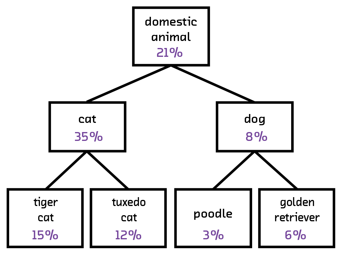
This step of augmenting the label predictions through a clustering scheme is incredibly important when dealing with potentially low confidence results. Since the data being sent to the model is often a lot more noisy than the original training dataset (which contained mainly stock photography) the actual accuracies we achieve on live data will be substantially less than what was advertised for the training data. Instead of hand-annotating live data in order to fine-tune the network with more realistic data we realized that, while sometimes the confidence in a classification was low, the network was generally pointing towards the correct concept. That is to say, even though there was no high confidence label for a given image of a dog, all of the dog-like labels had higher confidences than non-dog labels.
In doing the clustering, we are able to hide the low confidence in some classifications while still giving the user useful results. In the end, the user may not care whether we classify what type of dog is in the image but be more interested simply that there is a dog. Furthermore, having the taxonomy over the possible labels introduces a novel way of navigating through the dataset and gaining a deeper understanding of the landscape of images being taken.
Design and Deep Learning
By enabling increasingly accurate image object recognition and natural language processing, deep learning has the potential to open up new design possibilities for social web apps. The default organizational view for most social networks (e.g., Facebook, Twitter, Instagram) is the reverse-chronological feed, where posts are organized into topic-agnostic content blocks. Deep learning, by allowing designers to take the topic and sentiment of user posts into account, could enable new forms of organization and allow for designs that adapt themselves to better support different subjects and moods.
Beyond the Feed
In our prototypes we demonstrate how image object recognition can open up new paths of exploration in Instagram. While Instagram does have the capacity to group images together by category based on hashtags, uneven and idiosyncratic use of tags limits the effectiveness of this system-wide. [48] To have their pictures of a dog appear in the dog hashtag category, an Instagram user has to add ‘#dog’ to each one of the relevant photos. In Pictograph and Fathom this classification is taken care of, and thanks to our use of hierarchical tree classification that category is also automatically included under parent categories such as ‘animal’. Because we use image object recognition we don’t have to rely on users to input an image classification and can therefore include a much larger number of public images from the network in the relevant category page.
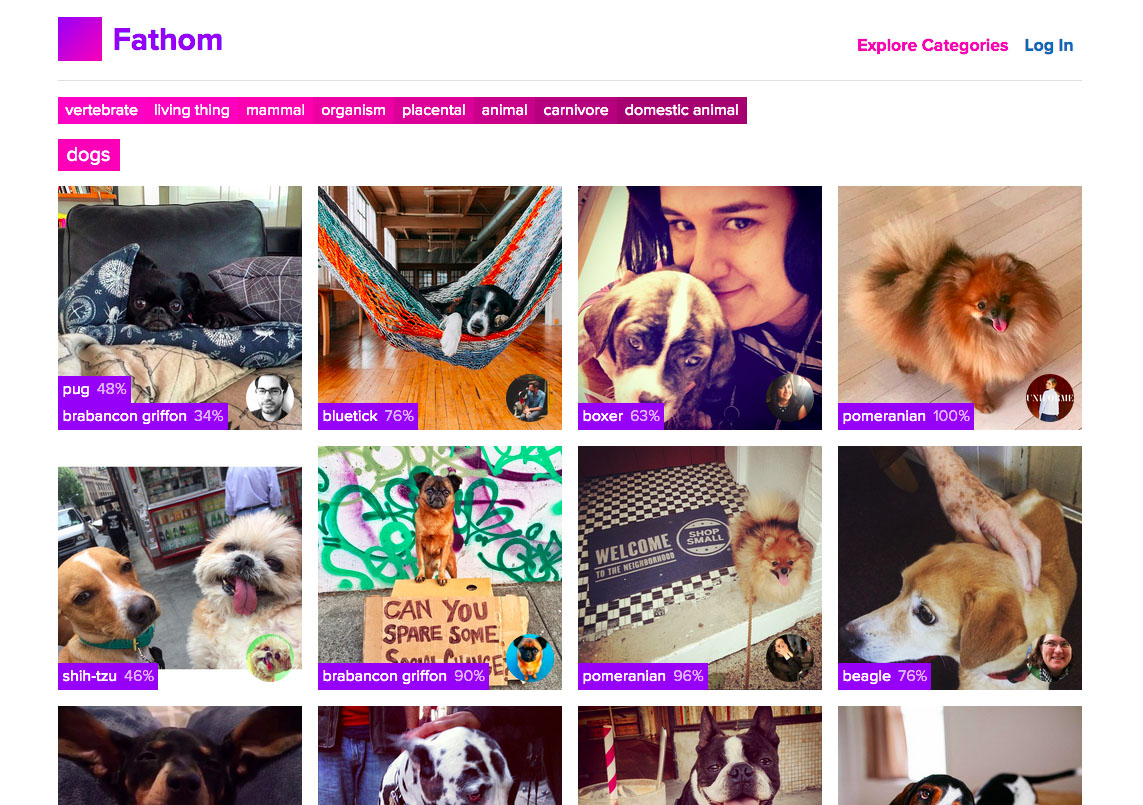
While our prototype focuses on the classifying possibilities of image object recognition. Other techniques powered by deep learning, such as natural language processing, could perform similar classifying and tagging operations for text-heavy posts. The capability to infer this kind of metadata from currently untagged user generated posts could greatly increase our ability to discover content by topic – a method of exploring that is intuitive to humans but up to now has been difficult to support at scale.
The information unlocked by deep learning will have to be integrated thoughtfully into current app design conventions. Better category classification could allow us to move away from reverse-chronological feeds – lengthening the lifespan of useful posts. The new info could also be used to improve the relevance of search results on social networks. These same qualities could also alter the moods of networks, however. Users may have become accustomed to old posts being buried in the stream or not readily visible to people outside their friends. For example, while most Instagram photos are public, for the non-celebrity the network can still feel like a very intimate place. If user photos are made more visible by improved classification features, such as the category pages in Fathom, that feeling of intimacy may be lost. Product creators will need to balance the increased access that deep learning can enable with user expectations.
While the ability to explore through category pages in Fathom can be seen roughly as an improvement to tagged category pages, the ‘Pictograph’ display, where a user’s top four most photographed categories are arranged as a proportional treemap, suggests some of the new visualizations that will be available as these technologies evolve.
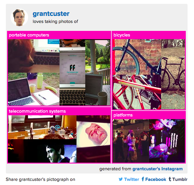
The pictograph visual moves toward saying something about the user’s personality based on classification. This possibility is only opened up when we have access to information about the content of a user’s images. [49]
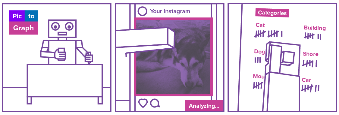
Paired with a hierarchical classifying system, this sort of classification could allow designs to adjust to support a user’s interests, or to build specially designed experiences around specific categories. Graphic designers who have access to the mood and content of a piece can design to support and enhance those elements. In the past this took the form of a designer being given a specific piece, in the future it might involve designing for specific mood and topic targets – where the content will then be matched to the design by a set of algorithmic classifiers. In this way, deep learning could support a return to content-specific design at a scale not previously possible.
Failed Prototypes
One common theme from people working with neural networks is the amount of failure when trying to build new systems. On the way to creating the Pictograph and Fathom prototype, we tried many things that simply did not work for one reason or another. One reason for this was the time limitation – as described in the <<devtimeline,development timeline>> section, creating new models can be time consuming. Another reason for this is availability of data – since we don’t have our own in-house datasets outside of data partnerships, finding the interesting and compelling problems for the datasets we have can be a challenge.
Below is a short list describing of some of the prototype ideas we were excited about but did not work. The recurring theme is the availability of data – many of the ideas were completely technically feasible however require access to clean data that was not easily attainable. Constant discussions were had regarding how to clean the data that we could get, from hand labeling to using Amazon Turk, however the cost of these methods couple with still not knowing if they would work turned us away from them. This serves as a testament to how important data quality is when creating neural systems.
Giphy
Giphy [50] is a search engine for animated GIFs. Animations are human annotated with tags that refer to the content of the animation with tags varying from “cat” to “cute” or “shock”. Our goal was to predict tags given an animation using video classification methods [51]. However, we faced many challenges when trying to create such a system.
The first challenge was dealing with the variability in GIF data. GIF’s have multiple standards that all deal with keyframing differently. This makes it so that when you are parsing an animation, great care must be taken to make sure the representations you have for each frame are correct and with minimal noise. In addition to simply extracting frames, many decisions had to be made for creating the neural system where framerates could be so variable. In general neural-video processing, it videos can be assumed to run at a standard framerate. GIF’s, on the otherhand, operate at a wide variety of frame rates (from 0.5 frame/second to 60 frames/second).
More importantly, however, was dealing with the quality of the tags. For typical image classification problems, the labels that are being extracted are very simple. Even when asking a human to do the comparable task, it is very simple to answer whether there is a dog in an image, but it is much more a matter of opinion whether an image portrays “shock” or “happy”. For a neural method to be able to make this identifications we need both a large set of examples in addition to a deep network in order to extract the relevant features.
In the end, we were not able to train a large enough model with the given dataset given our timeline. As discussed in the <<devtimeline,development timeline>>, neural networks have a large upfront time cost where you may understand what may be necessary for the model to work but it takes quite a long time to validate that hypothesis.
Nutrition
Seeing the wealth of images online of food, we also had the idea of creating a system which would take in an image of a dish and output the nutritional content of a dish. The plan was to find a repository with the nutritional content of various dishes, search for the dish on flickr [52] and train out model using this data.
The main problem with this attempt was the quality of the data. Here, since we were joining two different datasets (the nutritional content and the images of the food) the possibility for bad data was multiplied. Firstly, nutritional data for dishes is not very available. There are many sites that claim to provide the nutritional content of dishes (along with their recipes), however there are large discrepancies between what the sites report. This is probably because there are multiple ways to make a given dish, all of which contain slightly different ingredients and different quantities of them. In the end, one set of data was chosen as the “ground truth” simply because of the breadth of dishes that had data (including calorie, fat, protein, carbohydrates). This would also fare as a good benchmark for whether the system could work at all and whether it was worth it to put more time and resources in a potentially more accurate nutritional database.
Once we had some semblance of nutritional data we had to acquire images of each dish. The idea was to search flickr for the dish names along with certain phrases to select for images of food (such as “dish” and “food”). We keep the dish in our dataset if we were able to find 1,000 relevant images. However, upon doing a data quality check, it was evident that many pictures of a dish are of people cooking the dish as oppose to the final dish itself. This meant that many images of “burritos”, for example, were actually of a dish of rice or avocados that were being prepared for the final dish. In addition to simply being the wrong image for a given dish label, these images had overlap with other dishes (for example a salad) which further confused the neural network’s internal representation of the data.
In the end, data quality was the primary reason why this experiment failed. With images that were labeled under burrito that looked like a salad, pictures of a cutting board with a knife or a steaming pot for many of the dishes, and other such examples, there was no coherent features that could be extracted to discriminate between one dish or another. This problem persisted whether we tried to train a new neural network or frame it as a transfer task; as we trained the system we would constantly get wildly fluctuating results, an indication that the model couldn’t converge on relevant image features. Furthermore, we found out later that it is indeed possible – several days after we put this experiment away Google announced it had done a similar task of assigning caloric value to the image of a dish [53].
Ethics of Deep Learning
When we create a data product, we must consider not just the mathematical and computational aspects of the algorithm, but what the product experience of that algorithm feels like and the opportunities for it to go awry. Considering the worst-case scenario is not just something for Philip K. Dick and Ursula LeGuin; it must also be done conscientiously by engineers and product designers.
Deep Learning requires some creative thinking, for a number of reasons.
Uninterpretability
With Deep Learning, feature engineering is left to the algorithm. Therefore, you are never entirely certain what a specific feature represents, or even ultimately why the algorithm assigned the label that it produced. In machine learning we call this kind of algorithm uninterpretable.
Back in Section 2, we saw that neural networks learn by adjusting the weights and biases that connect and activate neurons. This simple strategy gives us great computational power, but reveals to us nothing about what any of these numbers or connections actually mean. That is, the underlying heuristics are nearly impossible to interpret. If the network encoded a feature based on race, there would be no easy way to figure this out or correct it. It is analogous to how neuroscientists and philosophers can’t discover properties of consciousness by simply looking at brain scans. This is a particular concern for companies working in highly regulated industries.
These risks are on the radar of many government and business leaders. Consider White House Counselor John Podesta warning students at the UC Berkeley School of Information, “We have a strong legal framework in this country forbidding discrimination based on [race, ethnicity, religion, gender, age, and sexual orientation] criteria in a variety of contexts. But it’s easy to imagine how big data technology, if used to cross legal lines we have been careful to set, could end up reinforcing existing inequities in housing, credit, employment, health, and education.” [54]
This is not a purely theoretical concern. Google’s image recognition software recently tagged two people of color as “gorillas,” and labeled a photo of the concentration camp at Auschwitz as a “jungle gym”. [55] Unfortunately, due the complexity of the system, the quick fix for the former offensive result was to simply eliminate the “gorilla” tag from the system entirely.
Uninterpretable systems are also vulnerable to propagating biases in the original source data. In one example, an ad server was observed advertising more higher-paying jobs to men than to women. [56] It’s extremely doubtful that any engineer designed that interaction, but it’s important to acknowledge the possibility of a system that uses gender, ethnicity, or socioeconomic status as a proxy for potential success in a highly abstracted feature space.
There is a further threat of having a system that does not have an inherent bias, but merely misinterprets a profile due to constraints in understanding context (see Section 2 for more on this). Take as an example those who are unjustly investigated and sometimes even prosecuted for crimes due to perceived “involvement” because they have family or friends that are involved in criminal activity. We see this as unethical because one cannot help where one is born, and thus one’s family and, to some extent, choice of friends. However, the issue here is that the data and profile surrounding the innocent person look a lot like those of the individuals involved in the crimes. Again we find a scenario in which neural networks could fundamentally misinterpret someone whose profile looks like it matches a certain classification. The consequences of such a misinterpretation must be considered carefully as delivery of such a system proceeds.
Some data leaders have recently proposed a method of “bias testing” that would develop metrics for evaluating and monitoring the likely bias of a deployed model. This is an active area of discussion and research.
Edge Cases: Liability and Error
Even with a model that is mathematically near perfect, there may be product consequences. Current Deep Learning systems typically achieve accuracy rates from 80-95%. But what about the >5% of results that are wrong?
Some examples of this kind of unfortunate edge case are Google’s data-driven overestimation of the scope of the influenza risk during the winter of 2012-2013, which left hospitals and clinics underprepared, [57] Facebook’s Year in Review showing a user photos of his recently deceased daughter, [58] and neural networks that mislabel images due to human-imperceptible distortions. [59]
As we enter a world where more neural networks are doing work across our business, state, and private ecosystems, we must take seriously the potential of an edge case causing serious harm. We are already seeing businesses forced to apologize publicly or settle cases due to social or emotional traumas inflicted upon individuals. We expect these incidents to occur more frequently as more products enter the market. Most of these technologies have obvious benefits – medical diagnoses, predictive traffic modeling, maintenance prediction – but the cost of an incorrect outcome may be monumental and it is unclear where the liability lies.
Unethical Applications
As this report is being written, The Future of Life Institute has already received signatures from over 1,000 robotics and AI researchers petitioning for a global ban on the development of weaponized AI. This intersects directly with the development of Deep Learning, since computer vision and classification would both be major components of any intelligent weaponry. While these technologies could be very good at their intended purposes and sometimes put people out of harm’s way, the potential to do bad seems high. This is an ongoing subject of debate among academics and people in the field.
If we zoom out from this stigmatized issue, we can find other application areas that carry similar face-value problems. Take for instance the possibility of a neural network that could profile online users or customers as vulnerable sales targets for high-interest loans. Given the data financial institutes have, this would be a fairly straightforward application for training a neural network. Yet, we recognize this as an unethical business practice that takes advantage of asymmetries in information and unfairly leverages socioeconomic data to place emotional pressure on people who want a better life. There have already been applications showing the possibility of this type of threat, such as Google advertising jail bonds to people with traditionally African-American names [60] and Facebook’s recent patent to help lenders do loan discrimination based on the applicant’s social network connections. [61]
We can find many examples where data is available to train a neural network to do something of questionable moral value. Price discrimination could easily be implemented by learning from online profiles and guessing the maximum price to display to a consumer. More insidious practices can be imagined where neural networks are trained to identify people taking part in protests, to deanonymize account information, or to discover personal vulnerabilities. In each of these cases, the application of a neural network provides one party with exploitative influence over another due to asymmetric access to or ownership of data.
What You Can Do
There are a few strategies used in the industry for avoiding these issues. The most basic and important of these strategies is taking appropriate time to consider the impact your system may have on a user – that is, having a good answer to the question, “What does it mean to a user if our system is wrong?” Preemptively recognizing edge cases and having an increased awareness of failure will help prevent surprises and improve the expectations of the users. It is expensive to train and retrain Deep Learning models, so reasonable forethought can save time and energy later.
Of course, these limitations cannot always be known in advance, but prepared engineering teams will always test their systems against diverse inputs. This is where considering a combination of edge cases and consequences alongside a robust testing protocol goes a long way. Testing your data against the unexpected user, or even the contrived worst-case scenario, will reveal a lot about the expected performance of the system and the potential errors. This is all good hygiene for robust systems.
The Future
Looking ahead, neural networks show a lot of promise to become widely used tools in many kinds of products and systems. More than other areas of AI, the potential for them to grow is very high. This is because, unlike other areas of AI and machine learning, once a model has been trained it will be very simple to take an out-of-the-box system and incorporate it into a larger service. Even more important, the ability to take a highly-tuned model and merely swap out a single layer and re-train it to fit a new problem (this is called a transfer task which we’ll explore in depth below) will lower the barrier to making useful systems.
The exact path into the future will depend on progress in several complimentary technologies (namely GPUs). Regardless, there are a number of promising applications and emerging areas that seem guaranteed to be influential in the coming years. Through this section we will outline a number of those and attempt to shed some light on where the future road of neural networks will take us.
Future of Academic Research
Serving as an extension of the current research, many types of extended convolutional neural network models have been created in order to solve specific problems or to extend the utility of the original model. Firstly, current convolutional neural networks operate on images that are approximately 227 x 227 pixels. By increasing computational and algorithmic power of these systems, larger images can be analysed and potentially yield more accurate results. Furthermore, sparse multi-dimensional convolutional networks have been created which can work on arbitrary point-cloud data as opposed to a fixed image. By working on a point-cloud, information can be learned about 3D models. This could lead to major advances in robotic automation where a neural network powered robots could make inferences about the space it sees from its kinect-like sensors. In addition, there has been work on networks like SimNet which take the lessons learned from convolutional networks (such as parameter sharing and pooling) and extends them to new operations outside of convolutions. This will make it possible to apply such models on a much more diverse dataset as long as the appropriate convolution-like operation can be defined.
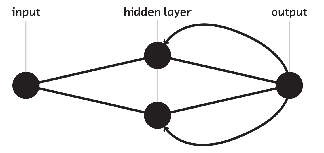
The technique with a more promising future is recurrent neural networks which allow a layer of neurons to have connections to any other layer regardless of its position in the network (this is the very thing that feed forward neural networks disallow). The ability to have backwards connections gives the network an understanding of temporal relationships which is important when doing sequence classification such as predicting the next word in a sentence or using multiple frames of a video to classify what is being shown. In fact, for robotics this sort of object classification is gaining more importance since it produces much less noise when doing object detection with a moving camera. Recurrent neural networks have also shown to produce very robust language models which can be used in a wide variety of applications, from tagging sentences, extracting entities in an article, to captioning images. In fact, the image captioning demonstration that was shown to the press used a convolutional neural network to feed into a recurrent neural network language model.
A beautiful aspect of recurrent neural networks is that they are Turing complete. This means that we can consider the trained weights of a recurrent neural network (RNN) to represent the definitions of a program that can compute anything that a normal computer could. It turns the form of backpropagation that runs on it into a pseudo-programmer that programs the RNN in order to solve a particular task. This may seem like a novelty, however the underlying theory of this proves the exceptional nature of RNN’s; while feed forward networks are universal approximators and can approximate any decidable problem, RNN’s are Turing complete and can fully compute any decidable problem!
Another subfield gaining popularity are transfer task oriented networks As
discussed in <
We are still a long way away from having very generalizable models that work on wide arrays of transfer tasks. However these tasks are becoming a larger part of deep learning research and at the same time we are gaining more “neural power” with recurrent neural networks. This makes us confident that recurrent neural networks with large focus on transfer tasks are the most promising avenue for the future of artificial intelligence.
Finally, very practically, there is work on making neural networks smaller and easier to compute. This work has multiple fronts, both on the hardware side in making GPUs more powerful and making the actual models smaller. One particularly interesting attempt at making the models smaller is to use lower precision numbers within the model (eg, storing 3.1 instead of 3.14159) [62]. This has the potential of simplifying the computational overhead of neural networks and making them more widespread on mobile and embedded devices.
2030: The World Deep Learning Built
On the road towards a more unified scheme for artificial intelligence, there will also be many intermediary capabilities which will bring the benefits of deep learning to many new fields.
There have recently been advances in turning sequences of 2D video frames into full featured 3D models of an environment. Although this is possible without a neural method, the current models are able to deal with noise and more exotic scenes much more robustly than previously possible. This has been quite a boon for robotics – it’s one thing for your roomba to be able to understand the layout of your space, but quite another to have it understand the objects, what they are and how to interact with them.

These sorts of alternate uses of convolutional layers of neural networks (eg, switching the fully connected layers from a convolutional neural network with other types of layers) have already been around for a couple years. For example, using Q-Learning [63] computers have been trained to learn how to play Atari games. [64] This training was done by simply letting the computer see the screen as a series of images, giving it a method of pressing buttons on the controller and also telling it what its current score is. This was enough for the system to learn how to interpret the gameplay and the relevant visual queues on screen in order to get a high score! [65] This sort of learning in which a computer learns the intricacies of a system and how to interact with it to get a desired outcome is incredibly exciting for robotics and control systems in general!
Another great innovation we are starting to see is the combination of linguistic models with other models. For example, recently we have been able to combine an image model with a recurrent language model in order to automatically and robustly caption images. [66] These captions are not templates or from a database, but rather a linguistic representation the model itself has created given an image! This sort of capability could be expanded for use in accessibility services for the blind or as a general-service natural language generation method.
On the other hand, the problem could also be inverted where language is the input and something else is the output. For example, a user could describe an object and have the model interpret the meaning and create the desired object. In the year 2050, will we simply tell our home computer that we’d like a vase to hold 12 flowers in the shape of a Klein bottle and have our in-house 3D printers hear that, create the model and print one for us?
We could also imagine applications where image processing is advanced to a degree where it can understand subtleties that currently require human experts. For example, a system could be built that takes in video frames from someone’s phone and helps them diagnose problems with their cars. As the network builds predictions, it can be fed back to the user as a request to zoom into particular parts of the car for further inspection. We are already seeing this sort of trend in expert neural network systems in the field of healthcare where data is already in a computer-usable format. In that field, neural networks are taking in MRI data, along with patient data, in order to aid doctors in diagnosis.
Conclusion
Deep Learning gives us the ability to analyze the contents of rich media, and, for the first time, gain insight into what is actually inside of those objects. We are just at the beginning of understanding how this set of techniques will be useful, and the results are already impressive. We can scan a social network and show you where people are disproportionately taking photos of oceans or mountains, look at your genomics or radiology data and make cheap and better healthcare recommendations, and find that photo of Aunt Margaret that you scanned in from a shoebox with one simple query.
We are more optimistic for the future development of Deep Learning than for any other form of machine learning. While this report specifically explores image analysis, we will soon see these techniques applied in other areas, and we believe this text provides a sound introduction to the principles necessary to understand and utilize modern neural networks.
In this report we have explored the history and mathematical foundations of the field, along with current applications and a survey of companies and open-source products that are in the market today. We’ve also speculated about what the near future holds. In the longer term, the ability for an algorithm to do feature engineering without the assistance of an engineer has the potential to change the way we build data processing systems. Even if image object analysis is irrelevant to your interests, this underlying change in how we conceive and engineer algorithms will impact your work.
In our prototypes, Pictograph and Fathom, we have demonstrated the utility of current image analysis techniques on a corpus of social photo data. This is interesting because the data is interesting – we are gaining new insight into human behavior through the lens of our collective desire to take smartphone photographs – but it is also a strong demonstration of the merits and challenges of these algorithmic techniques: we know if you’ve taken a photo of a Beagle puppy, but we don’t yet know if you were sad while you were doing it.
We remain optimistic for the future of Deep Learning, not just for image analysis, but for a variety of applications across industries. We expect to see this technique used for many more applications in a variety of industries over the next couple of years, and to see more breakthrough capabilities emerge from this research in the years beyond that.
Common choices for this function are
tanh, Softmax (i.e., generalized logistic regression), or ReLU. ↩︎For a good in-depth treatment of backpropagation, check out http://neuralnetworksanddeeplearning.com/chap2.html. ↩︎
For an in depth treatment of regularization see http://neuralnetworksanddeeplearning.com/chap3.html ↩︎
For a good treatment on convolutional neural networks, check out http://colah.github.io/posts/2014-07-Conv-Nets-Modular/ ↩︎
For a nice interactive aid in understanding convolutions, check out http://setosa.io/ev/image-kernels/ ↩︎
See Section 3 in http://arxiv.org/pdf/1404.7828.pdf ↩︎
See e.g. http://arxiv.org/abs/1506.02078 or http://arxiv.org/abs/1412.0035. ↩︎
https://en.wikipedia.org/wiki/Artificial_general_intelligence ↩︎
Further reading on this topic can be found at https://timdettmers.wordpress.com/2015/07/27/brain-vs-deep-learning-singularity/ ↩︎
http://caffe.berkeleyvision.org/gathered/examples/finetune_flickr_style.html ↩︎
To see the process in AWS, check out http://tleyden.github.io/blog/2014/10/25/cuda-6-dot-5-on-aws-gpu-instance-running-ubuntu-14-dot-04/ ↩︎
Who hasn’t wished for a real-life Douglas Adams Babel fish? ↩︎
See https://research.facebook.com/blog/814042348693053/fair-opening-up-about-artificial-intelligence-and-facial-recognition/. ↩︎
though not without controversy: see http://mashable.com/2015/05/21/flickr-auto-tagging-errors/ ↩︎
Make sure to download the version of
caffefrom NVIDIA’s GitHub repo, as well as their specialized math libraries, in order to take advantage of these optimizations. ↩︎https://github.com/BVLC/caffe/tree/master/models/bvlc_googlenet ↩︎
A hypernym is “a word with a broad meaning that more specific words fall under; a superordinate. For example, color is a hypernym of red.” ↩︎
While there aren’t numbers for Instagram, on Twitter hashtags are only used on 24% of tweets https://blog.bufferapp.com/10-new-twitter-stats-twitter-statistics-to-help-you-reach-your-followers. ↩︎
Again, hashtags could conceivably be used to perform a similar function, but real-world use of them is rarely consistent enough to support such a project. ↩︎
http://www.popsci.com/google-using-ai-count-calories-food-photos ↩︎
http://m.whitehouse.gov/sites/default/files/docs/040114_remarks_john_podesta_big_data_1.pdf ↩︎
http://www.theguardian.com/technology/2015/jul/01/google-sorry-racist-auto-tag-photo-app ↩︎
http://www.nature.com/news/when-google-got-flu-wrong-1.12413 ↩︎
http://www.theguardian.com/technology/2014/dec/29/facebook-apologises-over-cruel-year-in-review-clips ↩︎
http://techcrunch.com/2013/02/05/googles-unintentionally-racist-ads-probably-have-awful-psychological-impacts/ ↩︎
http://venturebeat.com/2015/08/04/facebook-patents-technology-to-help-lenders-discriminate-against-borrowers-based-on-social-connections/ ↩︎
For a demo of a comparable system, see: http://cs.stanford.edu/people/karpathy/convnetjs/demo/rldemo.html ↩︎